1. FINC4101 Investment Analysis
Instructor: Dr. Leng Ling
Topic: Portfolio Theory II

2. Learning objectives
Explain the benefit of diversification and identify the source of this benefit.
Understand the concepts of covariance and correlation.
Compute covariance and correlation between two risky assets.
Compute the expected return and standard deviation of a portfolio of two risky assets.
Define the minimum variance portfolio and compute its weights in the 2-risky asset case.
Define the investment opportunity set and the efficient frontier.
Overall objective: At the end of this topic, you should know something about how to form a portfolio of assets and why you should do it.

3. Learning objectives
Compute the expected return and standard deviation of a portfolio consisting of a risky asset/portfolio and a risk-free asset.
Define the Capital Allocation Line.
Define and compute the reward-to-variability (Sharpe) ratio.
Define the tangency portfolio and compute its weights in a 2-risky asset case.
Describe the process of efficient diversification with many risky asset and a risk-free asset.
Understand the idea of the separation property.

4. Portfolio Theory II: Concept Map
Diversification
Covariance,
Correlation
Efficient frontier
Property
Separation

5. This is the basic benefit of diversification.
Why diversify?
To reduce risk.
This is the basic benefit of diversification.
Tell student that we will demonstrate this point in the examples.

6. How does diversification work?
By exploiting the way different assets relate to each other.
We use a statistical measure called covariance to characterize the tendency of two assets to “move” with each other.
Covariance: A measure of the extent to which the returns of two assets tend to vary with each other.
An equivalent and easier to interpret measure is the correlation coefficient.
Correlation coefficient is simply the covariance divided by the product of the standard deviations of the returns on each asset.

7. Simple example
Consider two assets: a stock and a bond. There are 3 possible scenarios over the coming year:
HPR (%)
Scenario
Probability
Stock
Bond
Recession
0.3
-11 16
Normal
0.4 13 6
Boom 27 -4
Expected return 10
S.D.
14.92
7.75
The key determinant of portfolio risk is the extent to which the returns on the two assets tend to vary either in tandem or in opposition. Portfolio risk depends on the correlation between the return of the assets in the portfolio. We can see why with a simple 2-asset example.
The expected returns and S.D. are consistent with the scenario analysis data. Suppose we form a portfolio with 60% invested in the stock and 40% invested in the bond. See next slide

8. Portfolio of 60% in stock & 40% in bond
What is the expected return and S.D. of this portfolio?
Scenario
Prob.
HPR %
X HPR
Deviation from E( r )
Squared deviation
Prob. X squared deviation
Recession
0.3
-0.2
-0.06
-8.60
73.96
22.188
Normal
0.4
10.2
4.08
1.80
3.24
1.296
Boom
14.6
4.38
6.20
38.44
11.532
E( r )
8.40
Variance
35.016
S.D.
5.92
Tell students how to portfolio return in each scenario is computed.
Portfolio rate of return = weighted average of returns on each asset with weights equal to the proportion of the portfolio invested in each fund.
E.g., return in recession = 0.6 x (-11) x (16) = -0.20%

9. Diversification lowers risk!
Compare the standard deviations of the stock, bond and portfolio:
The portfolio is actually less risky than either of the two assets. Diversification lowers investment risk.
Why? Stock and bond returns tend to move in opposition to each other.
How do we measure this tendency? Covariance
Stock
Bond
Portfolio
14.92%
7.75%
5.92%
Make this clear to students: This simple example illustrates the power of diversification. In this instance, the portfolio sd is actually less than that of either asset. This shows that diversification – forming a portfolio – can lower investment risk.
The next question is how does this tremendous risk reduction come about?
The low risk of the portfolio is due to the inverse relationship between the performance of the two assets. In a recession, stocks fare poorly, but this is offset by the good performance of the bond fund. Conversely, in a boom scenario, bonds fall, but stocks do well. Therefore, the portfolio of the two risky assets is less risky than either asset individually. Portfolio risk is reduced most when the returns of the two assets most reliably offset each other.
The natural question investors should ask is how can one measure the tendency of the returns on two assets to vary either in tandem or in opposition to each other. The statistics that measure this tendency are the covariance and the correlation coefficient.

10. Deviation from mean return
Covariance
Deviation from mean return
Covariance
Scenario
Prob.
Stock
Bond
Product of Dev
Prob. x Product of Dev
Recession
0.3
-21 10
-210
-63
Normal
0.4 3
Boom 17
-10
-170
-51
-114
Recall that expected return of stock is 10%, expected return of bond is 6%.
In recession, stock return is -11, so deviation from mean = -11 – 10 = -21. The other entries are computed in a similar fashion.
The table shows the inner workings of covariance: the product of deviations is negative if one asset performs well when the other is performing poorly. It is positive if both assets perform well or poorly in the same scenario.
Use the table to show students how to actually compute covariance. Covariance is the probability-weighted average of the product of asset deviations from their respective means. To repeat, covariance measures the extent to which the returns of two risky assets tend to vary either in tandem or in opposition to each other.
The negative value of the covariance indicates that the two assets vary inversely, when one asset performs well, the other tends to perform poorly.

11. Covariance formula
Suppose there are S possible scenarios (i = 1,2,…,S), and the probability of scenario i is p(i), then covariance between assets A and B is
E(rA) = expected return of asset A; E(rB) = expected return of asset B
Interpreting the covariance: Cov > 0: two assets tend to move in tandem with each other. When one asset performs well (poorly) the other tends to perform well (poorly).
Cov < 0: two assets tend to move in opposition to each other. When one asset performs well (poorly) the other tends to perform poorly (well).
Cov = 0: two assets behave independently of each other. Knowing how one asset performs does not provide any information about how the other asset will perform.
Asset A’s return in scenario i
Asset B’s return in scenario i

12. Apply covariance formula
Go back to the example, but now suppose the returns on the stock are -14%, 13% and +30%. Compute the stock’s expected return, variance, and covariance with bond.
HPR (%)
Scenario
Probability
Stock
Bond
Recession
0.3
-14 16
Normal
0.4 13 6
Boom 30 -4
Expected return ?
S.D.
7.75
From Chp 6 EOC Q3/
Simple exercise on mean, variance and covariance.
Mean = (0.3 x -14) + (0.4 x 13) + (0.3 x 30) = = 10%
Variance = (0.3 x 576) + (0.4 x 9) + (0.3 x 400) = 296.4, SD = 17.22%
Covariance = 0.3 x (-14-10) x (16-6) x (13-10) x (6-6) x (30 – 10) x (-4 -6)
= – 60 = -132
Comparing the covariance with the one we have previously, we see that covariance has become more negative. Covariance has increased because stock returns are more extreme in the recession and boom periods. This makes the tendency for stock returns to be poor when bond returns are good (and vice versa) even more dramatic.

13. Correlation between assets A & B, rAB , is
Given this formula, we can write covariance as
Going back to our example, the correlation between stock and bond = -114/(14.92 x 7.75) = -0.99
Unfortunately, it is difficult to interpret the magnitude of the covariance. For instance, in our example, does the covariance of -114 indicate that the inverse relationship between the returns on stock and bond is strong or weak? It’s hard to say.
The correlation coefficient avoids this problem. Like covariance, the correlation coefficient also measures the tendency of two assets to co-vary, in addition it improves upon the covariance by telling us the strengthen of the tendency to co-vary.

14. Interpreting the correlation coefficient
Correlations range from -1 to 1.
Correlation
Meaning
-1, Perfect negative correlation
Strongest tendency for two assets to vary inversely/ move in opposite direction.
+1, Perfect positive correlation
Strongest tendency for two assets to move in tandem.
0, Uncorrelated
Returns on the two assets are unrelated to each other.
When correlation coefficient is 0, the returns of the two assets vary independently of each other.

15. Three rules of two-risky asset portfolio
Suppose you have a portfolio consisting of two risky assets, A and B. You invest the proportion, wA, of the portfolio in A and the proportion, wB , in B.
You know the following:
The return on asset A is rA ; the return on asset B is rB.
The expected return on asset A is E(rA) ; the expected return on asset B is E(rB).
The standard deviation of A is sA; the standard deviation of B is sB.
The correlation coefficient between the returns of A and B is rAB.

16. Rule 1: Portfolio rate of return
A portfolio’s rate of return (rP) is a weighted average of the returns on the component assets, with the investment proportions as weights,
rP = wA rA + wB rB
We have actually gone through all these in the preceding example. Tell students that. The formulas simply formalize and generalize the properties we encountered in the example.

17. Rule 2: Portfolio expected return
A portfolio’s expected return is a weighted average of the expected returns on the component assets with the same portfolio proportions as weights,
E(rP) = wA E(rA) + wB E(rB)

18. Rule 3: Portfolio variance
A portfolio’s variance (sP2) is
sP2 = (wAsA)2 + (wBsB)2 + 2(wAsA) (wBsB)rAB
Since cov(rA,rB) = sAsBrAB , we can also write portfolio variance as
sP2 = (wAsA)2 + (wBsB)2 + 2wAwBcov(rA,rB)
Taking the square root of sP2 gives us the portfolio standard deviation.
The variance of the portfolio is a sum of the contributions of the component asset variances plus a term that involves the correlation coefficient (and hence, covariance) between the returns on the component assets. If the correlation between the component assets is small or negative, then there will be a greater tendency for the variability in the returns on the two assets to offset each other. This will reduce portfolio risk. From the variance equation, we see that portfolio variance is lower when the correlation coefficient is lower (e.g., when correlation is negative).

19. Applying these rules Verify that:
Suppose you have two assets (A,B) with the following details:
E(rA)=6%, E(rB)=10%, sA=12%, sB=25%, rAB=0
wA = 0.5
Verify that:
portfolio expected return is 8%
portfolio SD is 13.87%
This example shows (1) the gain from diversification and (2) application of E( r ) and Var formulas.
The example involves shifting the portfolio from 100% invested in A to 50% invested in A and B.
Work through calculation in class.
E(rp) = (6 x 0.5) + (10 x 0.5) = = 8%
Var(rp) = (0.5x12)2 + (0.5x25)2 + 2 x (0.5 x 12) x (0.5 x 25) x 0 =
SD = (192.25)0.5 = 13.87%
Important discussion: the example shows that by investing in two assets the portfolio SD is actually smaller than the average of the 2 assets’ SDs.
If you don’t know about how portfolio variance is calculated and thus don’t appreciate the significance of covariance (correlation, assets offsetting each other and thus reducing volatility), then you might mistakenly compute portfolio SD as the average of the two assets’ SDs = ( )/2 = 18.5.

20. Discussion
By investing in two assets, the portfolio volatility is smaller than the average of volatilities of the two assets.
Why not use SD=(12+25)/2=18.5%?

21. Minimum variance portfolio
Weight on asset A is:
Weight on asset B is = 1 – wA.
Using this formula, verify that the min variance portfolio has wA=81.27%, wB=18.73%.
The previous slide shows us that we can reduce portfolio variance by combing assets. In fact, we can do better. We can actually work out the investment proportions that will produce a portfolio with the smallest possible variance. This portfolio is called the minimum variance portfolio. The formula is given on this slide.
Min variance portfolio weights.
wA = 252 – (12 x 25 x 0) / – (2 x12 x 25 x 0) = 252 / ( ) = 625/769 =
wB = 1 – = (When solving for weights, must express the weights as proportions, otherwise will not make sense).
Variance of the min variance portfolio = ( x 12)2 + ( x 25)2 =
SD of min variance portfolio = ( )0.5 = % [less than SD of the 50/50 portfolio, 13.87%]
Expected return = ( x 6) + ( x 10) = = 6.75%

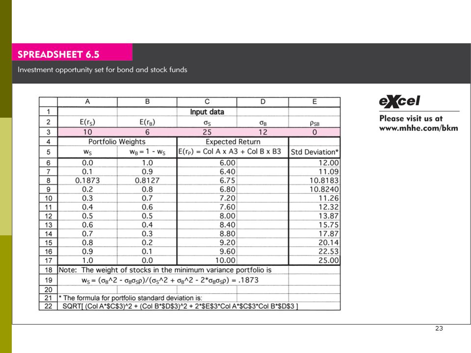
22. Investment opportunity set
The set of all attainable combinations of risk and return offered by portfolios formed using the available assets in differing proportions. B Z
So, we have just identified two portfolios that can be created with A and B: the 50/50 portfolio and the min variance portfolio. In fact, if we try out all possible combinations of the two assets and compute the expected return and SD of each combination, we will have the Investment opportunity set. Graphically, the investment opportunity set in this example is the graph on the slide.
Why should we be concerned with investment opportunity set? Imagine you are an investment advisor and you want to help your client choose a portfolio. You don’t know in advance which portfolio your client will choose. So the best you can do is to show your client all possible combinations of the assets (i.e., all possible portfolios) that your client can choose from, and let your client pick his preferred portfolio.
Talk a bit about how you can get the investment opportunity set in Excel (go to Portfolio Theory II workbook and show the spreadsheet ‘A,B investment opportunity set’. A

24. Mean variance criterion & the efficient frontier
Mean-variance criterion: choosing assets/portfolios based on the expected return and variance (or SD) of portfolios.
Using this criterion, we prefer portfolio A to portfolio B (or A dominates B) if:
E(rA)  E(rB) and sA  sB
Efficient frontier: portfolios on the upward sloping portion of the investment opportunity set.
There are many choices in the investment opportunity set. Choosing one portfolio is hard. Fortunately, there is a way to make our task easier. This is to eliminate some portfolios as they are inferior. The way to do this is to apply the ‘mean-variance criterion’. Define ‘mean-variance criterion’. Stress that the m-v criterion applies to both assets and portfolios. Recognize that an asset is just a portfolio with one asset. So there is no conflict.
Go back to the graph on previous slide and apply the rule. Show class that using the m-v criterion, investors would prefer asset B to asset Z because asset B has higher expected return and lower volatility. Also, point out that m-v criterion rules out portfolios that lie below the minimum-variance portfolio. Any portfolio on the downward sloping portion of the curve is “dominated” by the portfolio that lies directly above it on the upward sloping portion of the curve since that portfolio has higher expected return and equal standard deviation.
Using the m-v criterion, we rule out portfolios on the downward sloping portion and assets in the interior. The only portfolios worth considering are those on the upward sloping portion (in the northwest corner). Portfolios on the upward sloping portion constitutes the efficient frontier because they give the highest possible expected return for a given risk level or equivalently, they give the lowest possible risk for a given expected return (this includes min var portfolio). The idea of the efficient frontier is important because when we introduce a riskfree asset, the efficient frontier is formed by combining the riskfree asset with the tangency portfolio. This is what BMK calls the Capital allocation line. We will return to the idea of the efficient frontier later on.

25. Practice 2 Chapter 5: CFA problems: 4,7,8,9,11.
Chapter 6: CFA problems: 1, 3(a) only.

26. Homework 2
1. If required risk premium= , where A=4, and risk free rate = 1%, what are the annual required rates of return for the following investments? What will be the value of these investments after 2 years, if these investments have achieved the required return rates?
2. You are considering investing in 2 assets. A asset has an expected return of 15% and standard deviation of 32%. B asset has an expected return of 9% and standard deviation of 23%. The correlation between A and B is 0.15.
What is the covariance between A and B?
What is the weight of A and B in the minimum variance portfolio?
What is the expected return and variance of the minimum variance portfolio?
Investment
standard deviation
value today 1
0.4
$1,000 2
0.5 3
0.6 4
0.2

27. Extreme cases Suppose rAB= 1, sP2 = (wAsA + wBsB)2 sP = wAsA + wBsB
No gains from diversification only in this case!
Whenever r < 1, there are gains from diversification.
Suppose rAB= -1,
sP2 = (wAsA - wBsB)2
sP = ABS[ wAsA – wBsB ]
Correlation = 1
Portfolio standard deviation is a weighted average of component security std devs.
Whatever the proportions of stocks and bonds, both the portfolio mean and std dev are simple weighted averages.
With perfect positive correlation, the opportunity set is a straight line through the component securities. no portfolio can be discarded as inefficient and the choice among portfolios depend only on risk preference. Diversification in the case of perfect positive correlation is not effective.
Perfect positive correlation is the only case in which there is no benefit from diversification. Whenever correlation < 1, the portfolio s.d. is less than the weighted average of the standard deviations of the component securities. Therefore, there are benefits to diversification whenever asset returns are less than perfectly correlated. In fact, as the correlation becomes smaller and smaller (from positive, to zero to negative), the benefits increase. In the extreme, if two assets are perfectly negatively correlated (the extreme class), we can even completely reduce risk.
Correlation = -1
ABS = absolute value
Negative correlation between a pair of assets is also possible. When correlation = - 1, the portfolio std dev is the absolute value of wAsA – wBsB . The solution involves the absolute value because standard deviation is never negative. With perfect negative correlation, the benefits from diversification stretch to the limit. We can reduce portfolio std dev to 0. How? Substitute correlation = -1 into the min variance formula and solve for the asset weights. This will be the zero std dev portfolio.
Correlation of -1 is very extreme and rarely seen in real life. A realistic correlation between stocks and bonds based on historical experience is actually around 0.20.
On the next slide, we see the investment opportunity set for various correlations.

28. Investment opportunity set with different correlationsB A
Mention that when correlation=1 in our example (assets A and B), the opportunity set is a straight line, when correlation < 1, opportunity set becomes a parabola, and there are benefits to diversification. In the extreme when correlation = -1, the opportunity set consists of two lines, one going through A, the other going through B. The zero std dev portfolio is the one on the vertical axis.

29. Problem
Jane Marple has an $800,000 fully diversified portfolio. She subsequently inherits Rafael Aerospace Inc. stock worth $200,000. Her financial advisor provided her with the following information for the coming year:
The correlation between the original portfolio and Rafael Aerospace is 0.3.
Jane will keep the new stock. (a) Calculate the expected return and standard deviation of the new portfolio. (b) Calculate the covariance between the original portfolio and Rafael Aerospace.
Expected annual HPR (%)
Std Dev of annual return (%)
Original portfolio
6.7
9.3
Rafael Aerospace
8.2
15.6
Based on Chp 6 EOC Q5 (a)
First, find the portfolio weights (one of the most important things to do).
Total portfolio wealth = 800k + 200k = 1000k or 1,000,000
Weight of original portfolio = 800,000/1000,000 = 0.8
Weight of Rafael = 200,000/1000,000 = 0.2
Expected return = (0.8 x 6.7) + (0.2 x 8.2) = 7%
Std dev = [ (0.8 x 9.3)2 + (0.2 x 15.6)2 + 2(0.8)(0.2)(0.3)(9.3)(15.6) ]0.5
= [ ]0.5 = [ ]0.5
= = 8.9%
Again, show power of diversification. Get higher expected return, and lower SD.
For (b), just use the alternative formula for covariance = correlation x SD of original portfolio x SD of Rafael
= 0.3 x 9.3 x 15.6 =

30. Follow-up problems
Jane decides to keep Rafael Aerospace but wants to rebalance the new portfolio so that risk is reduced to the minimum. What are the weights, the expected return and std dev of the minimum variance portfolio?
Continuing with the previous problem, if Jane keeps the original composition, what is the portfolio expected return and SD if the correlation is (a) 1, (b) -1.
1) Introduce the terminology of ‘rebalance’ or ‘rebalancing’, which means changing the weights or composition of the portfolio, without changing the component assets.
Use the formula for the minimum variance portfolio to solve for the weight on original portfolio (labeled it as A)
WA = (15.62 – (9.3 x 15.6 x 0.3) )/( – (2 x 9.3 x 15.6 x 0.3))
= ( – )/( – )
= /
= = or 82.3%
Weight on Rafael, WB = 1 – = 17.7%
Expected ret of min var portfolio = (0.823 x 6.7) + (0.177 x 8.2) = = or 6.96%
Portfolio SD = [(0.823 x 9.3)2 + (0.177 x 15.6)2 + 2(0.823)(0.177)(9.3)(15.6)(0.3)]0.5 = or 8.88%
2) So now, weights are 80% on original, 20% on Rafael. The part on expected return is a trick question.
For (a) and (b), expected return is still 7% because the expected return formula only depends on weights and component asset expected returns. These have not changed, so expected return is unchanged.
But SD is different because correlation has changed.
(a) Portfolio SD = 0.8 x x 15.6 = 10.56% (make use of formula on slide 26)
(b) Portfolio SD = ABS[0.8 x x 15.6] = 4.32% (make use of formula on slide 26)

31. Asset allocation involving risky assets and a risk-free asset.
What’s a risk-free asset?
An asset that provides a sure (for certain) nominal rate of return. It is a default free asset. Examples:
U.S. Treasury securities (Treasury bills, Treasury notes, Treasury bonds),
Portfolios invested in these securities, e.g., T-bill money market fund.
In practice, money market instruments like bank certificate of deposits (CDs) and commercial paper are treated as effectively risk-free.
Treasury bills are also known as T-bills, Treasury notes are also known as T-notes, Treasury bonds are also known as T-bonds.
Why are Treasury securities risk free? Because the Federal government can raise taxes and print money to pay the debt (Treasury securities) when they mature. The power to tax and to control the money supply lets the government, and only the government, issue default-free (Treasury) securities.
The default free guarantee by itself is not sufficient to make the bonds risk-free in real terms, since inflation affects the purchasing power of the proceeds from an investment in T-bills. The only risk-free asset in real terms would be a price-indexed government bond. Even then, a default-free, perfectly indexed bond offers a guaranteed real rate to an investor only if the maturity of the bond is identical to the investor’s desired holding period.
In practice, money market instruments like bank certificate of deposits (CDs) and commercial paper are also treated as effectively risk-free. All the money market instruments are virtually immune to interest rate risk (unexpected fluctuations in the price of a bond due to changes in market interest rates) because of their short maturities, and all are fairly safe in terms of default risk (because the issuers are usually creditworthy companies).

32. Properties of risk-free asset
There is no uncertainty in return.
Variance of risk-free asset is 0
Likewise, standard deviation is 0
The risk-free asset does not vary with a risky asset/ portfolio. So,
Cov(risk-free asset, risky asset) = 0
Corr(risk-free asset, risky asset) = 0

33. 3 rules when there is one risk-free asset & one risky asset (1)
P: risky asset/ portfolio (wP) +
Risk-free asset (wf)
What is the correlation between P and the risk-free asset?
Complete portfolio, C P
Risk-free
Return rP rf
Expected return
E(rP)
S.D. sP
Suppose you have a portfolio consisting of a risky asset/portfolio, P, and a risk-free asset. The weight on the risky asset is wP, the weight on the risk-free asset is wf .
The entire portfolio of risky and risk-free assets is sometimes called the complete portfolio, denoted by C.
For risk-free, expected return is the same as the realized return.
What is the standard deviation of the risk-free asset? Ans: 0.
What is the correlation between P and the risk-free asset? Ans: 0.
Just an application of the previous slide.

34. 3 rules when there is one risk-free asset & one risky asset (2)
1) Portfolio return, rC = wP rP + wf rf
2) Portfolio expected return, E(rC) = wP E(rP) + wf rf
Portfolio risk premium, E(rC) - rf = wP [ E(rP) – rf ]
3) Portfolio variance, sC2 = (wPsP)2
Portfolio standard deviation, sC = wPsP
Derivation of portfolio risk premium,
E(rC) – rf = wP E(rP) + wf rf – rf = wP E(rP) + wf rf – (wP + wf )rf [make use of the fact that wP + wf = 1 ]
= wP E(rP) + wf rf – wPrf – wf rf
= wP E(rP) – wPrf
= wP [E(rP) – rf ]
Derivation of portfolio variance, 2 = (wPP)2 + (wf x 0)2 + 2(wP)(wf)(P)( 0 )( 0 ) = (wPP)2
Use the fact that std dev of risk-free is 0 and covariance is 0.
The risk premium and standard deviation of the complete portfolio increase in proportion to the investment in the risky portfolio. This makes sense since the risk of the complete portfolio only comes from the risky portfolio P. Basically, the higher the investment in P, the higher the risk (SD) and risk premium.

35. Capital Allocation Line (CAL)
If we plot the expected return and standard deviation combinations of a complete portfolio, we get the Capital Allocation Line (CAL).
CAL: The plot of risk-return combinations available by varying portfolio allocation between a risk-free asset and a risky asset/portfolio.
CAL is just the investment opportunity set when we have a risk-free asset and a risky asset/portfolio!
Capital Market Line (CML): the CAL when the market index portfolio is used as the risky portfolio.

36. Capital Allocation Line (CAL)

37. Apply these rules
Suppose the risky portfolio P has an expected return of 15% and a standard deviation of 22%. The risk-free asset promises a return of 7%.
Compute the expected return, risk premium and standard deviation of the complete portfolio if
100% of the portfolio is invested in P
100% of the portfolio is invested in the risk-free asset
Equal weight is placed on P and the risk-free asset.
Draw the CAL.

38. Results Expected return Risk premium Portfolio SD 100% in P
(1 x 15) + (0 x 7) = 15
1 x [15 – 7] = 8
1 x 22 = 22
100% in risk-free
(0 x 15) + (1 x 7) = 7
0 x [15 – 7] = 0
0 x 22 = 0
Equal weight
(0.5 x 15) + (0.5 x 7) = 11
0.5 x [15 – 7] = 4
0.5 x 22 = 11
When 100% is allocated to P, obviously, the portfolio C is just portfolio P. So not surprising the expected return and std dev of C are exactly the same as those of P.
When 100% is allocated to riskfree, the complete portfolio is just the riskfree asset. So the portfolio has 0 SD and expected return = riskfree rate.
When 50% is invested in each, the risk premium and SD of C is half that of P. when you reduce the fraction of the complete portfolio allocated to the risky asset by half, you reduce both the risk and risk premium by half.
Side note: The authors made the following point in Chp 5: if the risky portfolio is the market index portfolio then the CAL is called the Capital Market Line. What is the market index portfolio: it is the portfolio with all the stocks in a broad market index such as the S&P 500 index.
Capital Market Line: The capital allocation line using the market index portfolio as the risky asset.
However in Chapter 7, the authors define the CML as the CAL when the tangency portfolio is the market portfolio. The two definitions can be reconciled only if you believe the market index like the S&P 500 adequately represents the true unobserved market portfolio.

39. Capital Allocation Line (CAL)
Slope of CAL = increase in expected return per unit of additional standard deviation (SD), i.e., the extra return per extra risk.
The slope is also called the Sharpe ratio, reward-to-variability ratio.

40. S = portfolio risk premium / portfolio std dev
Sharpe ratio, S
Sharpe ratio is the slope, so use “rise” over “run”.
For our example, Sharpe ratio= (15 – 7)/(22 – 0)
= 8/22
= 0.36
In general, Sharpe ratio of portfolio
S = portfolio risk premium / portfolio std dev
Sharpe ratio is the same for all portfolios that plot on the CAL.
Since the Sharpe ratio is the slope of the CAL, we can make use of simple mathematics to compute the Sharpe ratio. Recall that slope = rise / run.
So using the two points: (0,7) [100% in riskfree], (22,15) [100% in P], then Sharpe ratio = 15 – 7/22 = 8/22 = 0.36
While the risk-return combinations differ, the ratio of reward to risk is constant.

41. Problems involving risk-free and risky assets
Assume you manage a risky portfolio with an expected rate of return of 17% and a standard deviation of 27%. The T-bill rate is 7%.
a) Your client invests 70% of his portfolio in your fund and 30% in a T-bill money market fund. What is the expected return and standard deviation of your client’s portfolio?
b) Suppose your risky portfolio includes the following investments in the given proportions:
What are the investment proportions of your client’s overall portfolio, including the position in the T-bills?
c) What is the Sharpe ratio of your risky portfolio and your client’s overall portfolio?
d) Draw the CAL and point the positions of your and your client’s portfolios.
Stock A
27%
Stock B
33%
Stock C
40%
E(rP) = (0.3 x 7%) + (0.7 x 17%) = 14% per year
SD = 0.7 x 27 = 18.9% b)
Investment proportion in A = 0.27 x 0.7 = or 18.9%
Investment proportion in B = 0.33 x 0.7 = or 23.1%
Investment proportion in C = 0.40 x 0.7 = 0.28 or 28%
Investment proportion in T-bills is 30%.
Sum = = 100%
c) Sharpe ratio of both portfolios is the same.
Your risky portfolio S = (17 – 7)/27 = 10/27 = 0.37
Client’s overall portfolio S = (14 – 7)/18.9 = 7/18.9 = 0.37
Client’s portfolio lies on the CAL with your risky portfolio.

42. Optimal risky portfolio with a risk-free asset
When we have risky assets and a risk-free asset, we can identify one single risky portfolio that gives us the highest possible Sharpe (reward-to-variability) ratio.
This risky portfolio is the ‘optimal’ or ‘tangency’ portfolio.
The CAL formed using the optimal risky portfolio has the steepest slope.
All risk-averse investors would prefer to form their complete portfolios using the risk-free asset with the optimal portfolio than any other risky portfolio. So the optimal portfolio dominates all other risky portfolio.

43. Recall: E(rA)=6%, E(rB)=10%, sA=12%, sB=25%, rAB=0.2.
Go back to the 2 risky assets: A and B but assume correlation is 0.2. Now add a risk-free asset with 5% return B
CAL2
CAL1 2 1 A
The pink investment opportunity set is the investment opportunity set formed using assets A and B which we have been using.
CAL1 is the CAL formed by combining risk-free asset with risky portfolio 1 (formed from A and B)
CAL2 is the CAL formed by combining risk-free asset with risky portfolio 2
CAL2 is steeper than CAL1 implying that portfolio 2 has a higher Sharpe ratio than portfolio 1. Combinations of portfolio 2 and the risk-free asset provide a higher expected return for any level of risk (standard deviation) than combinations of portfolio 1 and the risk-free asset. Therefore, all risk-averse investors would prefer to form their complete portfolio using the risk-free asset with portfolio 2 rather than portfolio 1. in this sense, portfolio 2 dominates portfolio 1.
We can continue this process of locating risky portfolio that will produce steeper and steeper CALs (i.e., CALs with higher and higher Sharpe ratios).
The risky portfolio that will produce the steepest possible CAL (highest possible Sharpe ratio) is the portfolio at the tangency point between the investment opportunity set and the line drawn from the risk-free rate of 5%. In our graph, the portfolio O is the risky portfolio at the tangency point. So combing portfolio O with the risk-free rate gives the CAL with the highest possible Sharpe ratio. This is the steepest possible CAL that can be produced with the feasible (available) risky portfolios.
This portfolio O is the optimal risky portfolio/ tangency portfolio. As mentioned on the previous slide, the CAL formed using O has the steepest slope.
Ok, so we have identified the optimal risky portfolio graphically. We can identify this portfolio analytically using the formula on the next slide.
Recall: E(rA)=6%, E(rB)=10%, sA=12%, sB=25%, rAB=0.2.

44. Optimal risky portfolio weights
Using the formulas, the weights in the optimal portfolio (O):
wA = 32.99%, wB = 67.01%
Expected return, SD, Sharpe ratio:
E(rO) = 8.68%
sO = 17.97%
SharpeO = (8.68 – 5)/17.97 = 0.20
These formulas are derived from the maximization of the Sharpe ratio.
Tell class that they don’t have to memorize. If tested, the formula will be given.
Show how the formula is used to obtained the weights, expected returns and standard deviations.
wA = [6 – 5](252) – [10 – 5](12 x 25 x 0.2) /([6 – 5](252) + [10 – 5](122) – [ ] (12 x 25 x 0.2)
= (252) – 300 / ((252) + 5(122) – 6 x 60)
= 325 / 985
= or 32.99%
wB = 1 – = or 67.01%
E(rO) = ( x 6) + ( x 10) = = 8.68%
O = [( x 12)2 + ( x 25)2 + 2(0.3299)(0.6701)(12)(25)(0.2)]0.5
= [ ]0.5
= = 17.97%

45. Risk aversion and portfolio choice
Preferred complete portfolio: 55% in Portfolio O, 45% in risk-free asset.
Identifying the tangency portfolio only allows us to the identify the collection of complete portfolios with the best reward-to-risk ratio (Sharpe ratio). However, each individual investor must still identify one single, most preferred complete portfolio from the CAL. How does the investor do this? Based on his risk-aversion.
The choice of the preferred complete portfolio depends on the investor’s risk aversion. More risk-averse investors will prefer low-risk portfolios despite the lower expected return, while more risk-tolerant investors will choose higher-risk, higher-return portfolios. Both investors, however, will choose portfolio O as their risky portfolio since that portfolio results in the highest return per unit of risk, i.e., the steepest CAL. Investors will differ only in their allocation of investment funds between portfolio O and the risk-free asset.
The graph shows one possible choice for the preferred complete portfolio, C.
The expected return = 5 + (0.55)[8.68 – 5] = 7.02%
SD = 0.55 x = 9.88%

46. Consider the following
A pension fund manager is considering 3 mutual funds. The first is a stock fund, the second is a corporate bond fund, and the third is a T-bill money market fund that yields a sure rate of 5.5%. The expected return and sigma of the risky funds are:
The correlation between the risky fund returns is 0.25.
Expected return
Std Dev
Stock fund (S)
14%
30%
Bond fund (B) 8 20

47. Answer the following:
1)Compute the expected return and standard deviation of the minimum variance portfolio.
2)Compute the expected return and standard deviation of the tangency portfolio.
3)What is the Sharpe ratio of the tangency portfolio?
4)Suppose you want to form a complete portfolio on the CAL. The portfolio must yield an expected return of 12%.
What is the standard deviation of the portfolio?
What is the proportion invested in the T-bill fund and each of the two risky funds?
1) Use the formula for the minimum variance portfolio weights.
wS = 202 – (20 x 30 x 0.25)/ ( – 2 x 20 x 30 x 0.25) = ( )/(1300 – 300) = 250/(1000) = 0.25
wB = 1 – 0.25 = 0.75
E(r) = (0.25 x 14) + (0.75 x 8) = 9.5%
SD(r) = [ (0.25 x 30)2 + (0.75 x 20)2 + 2(0.25)(0.75)(20)(30)(0.25) ]0.5 = [ ]0.5 = 18.37%
2) First, find weights of the tangency portfolio
wB = ([8 – 5.5](302) – [14 – 5.5](20)(30)(0.25) ) /([8 – 5.5](302) + [14 – 5.5](202) – [ – 2(5.5)](20)(30)(0.25) )
= (2250 – 1275)/( – [11 x 150])
= 975/(4000) = or %
wS = 1 – = or %
E(r ) = ( x 8) + ( x 14) = = = 12.54%
SD(r) = [( x 20)2 + ( x 30)2 + 2( )( )(20)(30)(0.25)]0.5 = = 24.37%
3) Sharpe ratio = (12.54 – 5.5)/24.37 = = 0.29 (to 2 d.p.) 4)
Two ways to do this:
Method 1:
Let y be the proportion in the tangency portfolio.
12 = y[12.54 – 5.5]
y = ( 12 – 5.5 )/[12.54 – 5.5] = 6.5/ 7.04 = or 92.33%
SD(r ) = x = = 22.50%
Method 2:
Use the fact that the complete portfolio’s Sharpe ratio is equal to the tangency portfolio’s Sharpe ratio.
Tangency portfolio’s Sharpe ratio = Set this equal to complete portfolio’s risk premium divided by its standard deviation.
= (12 – 5.5)/SD(r) => SD(r) = (12 – 5.5)/ = = 22.50% (to 2 d.p)
Proportion invested in t-bill fund = 1 – y = 1 – = or 7.67%
Proportion invested in bond fund = x = or 22.51%
Proportion invested in stock fund = x = or 69.82%
= 100%

48. Efficient diversification with many risky assets & a risk-free asset (1)
Efficient diversification entails 3 separate steps:
Form efficient frontier of risky assets
Efficient frontier: the collection of portfolios that maximizes expected return at each level of portfolio risk/ standard deviation.
Northwestern-most portfolios
Inputs: expected return and SD of every risky asset, plus correlation coefficients between each pair of assets.
So far, you have learnt the different components of an integrated process for efficient diversification.
Now, it’s time to re-cap and bring together all these different components.
Step 1) Form efficient frontier of risky assets. We looked at this on slides 22,23,24 when we discussed the mean-variance criterion. In fact, on slide 22, we talked about an efficient frontier when there are only two risky assets: A and B. Now, all that we are doing is generalizing the idea of more than two assets.
The expected return, standard deviations and correlations come from security analysis, i.e., equity valuation portion of the course.
Portfolios on the efficient frontier are “efficiently” diversified in the sense that they offer the highest possible expected rate of return for each level of portfolio standard deviation. The next slide shows an example of an efficient frontier.

49. Efficient frontier of risky assets
Inefficiently diversified. N W E
Make the following points:
1) Use the compass to show students why efficient frontier portfolios are the ‘northwestern-most’ portfolios.
2) Expected return-standard deviation combinations for any individual asset end up inside the efficient frontier, because single-asset portfolios are inefficient – they are not efficiently diversified.
3) When we choose among portfolios on the efficient frontier, we can immediately discard portfolios below the minimum-variance portfolio. There are dominated by portfolios on the upper half of the frontier with equal risk but higher expected returns. therefore, the real choice is among portfolios on the efficient frontier above the minimum variance portfolio.
Various constraints may preclude a particular investor from choosing portfolios on the efficient frontier, however. If an institution is prohibited by law from taking short positions in any asset, for example, the portfolio manager must add constraints to the compute optimization program that rule out negative(short) positions. Besides short-sale constraints, other constraints include constraint on a minimum level of dividend yield.
Nowadays, there are computerized packages which compute the efficient frontier given a collection of risky assets. In fact, you can also do it with Excel. Show the efficient frontier in the excel file, “excel_app_Chapter_06_Efficient_Frontier_for_Many_Stocks.xls”.
Portfolios are discarded. Dominated by portfolios on efficient frontier. S

50. Efficient diversification with many risky assets & a risk-free asset (2)
Use the risk-free rate and efficient frontier to find the tangency portfolio or optimal risky portfolio
Recall that the tangency portfolio gives us the CAL with the highest Sharpe ratio
Investor chooses the preferred complete portfolio based on his/her risk aversion.
Each investors will use tangency portfolio in forming his/her complete portfolio
2) We went through the process of finding the tangency portfolio on slides The same steps apply but now we have to broaden it to more than two stocks.
Finding the tangency portfolio is also within the capability of a spreadsheet program. You would are doing is to find the vector of the complete portfolio weights which maximize the Sharpe ratio.
Risk-free asset is usually the t-bill.
3) The investor chooses the appropriate mix between the optimal risky portfolio (O) and the risk-free asset. A portfolio manager will offer the same tangency portfolio to all clients, no matter what their degrees of risk aversion. Risk aversion comes into play only when clients select their desired point on the CAL. More risk-averse clients will invest more in the risk-free asset and less in the tangency portfolio than less risk-averse clients, but both will use the tangency portfolio as the optimal risky investment vehicle.
This result is called a separation property introduced by James Tobin. The property implies that

51. Separation Property
The act of choosing the appropriate portfolio can be separated into two independent tasks.
Find the optimal risky portfolio.
This consists of steps 1 and 2 and is a purely technical problem.
Given the input data, the best risky portfolio is the same for all clients regardless of risk aversion.
Investor constructs complete portfolio using risk-free asset and optimal risky portfolio.
Depends on the investor’s risk/personal preference. Here the client is the decision maker.
Introduced by James Tobin
The separation property implies that portfolio choice can be separated into two independent tasks.
When will the separation property not be true?
1) The optimal risky portfolio for different clients may vary because of portfolio constraints such as dividend yield requirements, tax considerations, or other client preferences.
2) If different portfolio managers use different input data to develop different efficient frontiers, they will offer different “optimal” portfolios. Therefore, the real arena of the competition among portfolio managers is in the sophisticated security analysis that underlies their choices. The rule of GIGO applies fully to portfolio selection. If the quality of the security analysis is poor, a passive portfolio such as a market index fund can yield better results than an active portfolio tilted toward seemingly favorable securities.

52. Summary Efficient diversification reduces risk.
Benefit of diversification depends on how assets co-vary with each other.
Efficient frontier is the collection of portfolios offering the highest expected return for each level of risk.
Introducing a risk-free asset allows us to identify the tangency portfolio and the CAL.
Tangency portfolio has the highest Sharpe ratio and therefore is most desirable.
Implications of the separation property.

53. Practice 3
Chapter 5: 13,14,18,19.
Chapter 6: 8,9,10,11,12,19.

54. Homework 3
Assume you manage a risky portfolio with an expected rate of return of 20% and a standard deviation of 30%. The T-bill rate is 5%. Your client invests 60% of his portfolio in your fund and 40% in a T-bill money market fund. What is the expected return and standard deviation of your client’s portfolio? What is the Sharpe ratio of your client’s portfolio?
A asset has an expected return of 20% and standard deviation of 30%. B asset has an expected return of 10% and standard deviation of 23%. C asset is risk-free with a rate of 5%. The correlation between A and B is a) What is the expected return and standard deviation of the optimal risky portfolio? b) Suppose your complete portfolio must yield an expected return of 15% and be efficient. What is the standard deviation of your portfolio? c) What is the proportion of your portfolio invested in A and B, respectively?