Download presentation
Presentation is loading. Please wait.

1
Artificial Neural Networks
Wismar Business School Artificial Neural Networks Uwe Lämmel

3
Literature & Software Robert Callan: The Essence of Neural Networks, Pearson Education, 2002. JavaNNS based on SNNS: Stuttgarter Neuronale Netze Simulator

4
Prerequisites NO algorithmic solution available or algorithmic solution too time consuming NO knowledge-based solution LOTS of experience (data) Try a NN
 Try a NN.")
5
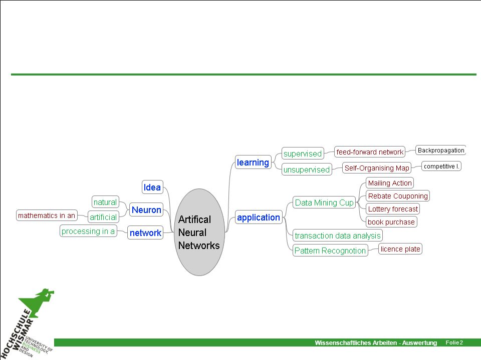
Content Idea An artificial Neuron – Neural Network
Supervised Learning – feed-forward networks Competitive Learning – Self-Organising Map Applications

6
Two different types of knowledge processing
Logic Conclusion sequential Aware of Symbol processing, Rule processing precise Engineering „traditional" AI Perception, Recognition parallel Not aware of Neural Networks fuzzy Cognitive oriented Connectionism

7
Idea A human being learns by example “learning by doing”
seeing(Perception), Walking, Speaking,… Can a machine do the same? A human being uses his brain. A brain consists of millions of single cells. A cell is connected with ten thousands of other cell. Is it possible to simulate a similar structure on a computer?
, Walking, Speaking,… Can a machine do the same A human being uses his brain. A brain consists of millions of single cells. A cell is connected with ten thousands of other cell. Is it possible to simulate a similar structure on a computer")
8
Idea Artificial Neural Network
Information processing similar to processes in a mammal brain heavy parallel systems, able to learn great number of simple cells ? Is it useful to copy nature ? wheel, aeroplane, ...

9
Idea An artificial neural network functions in a similar way a natural neural network does. we need: software neurons software connection between neurons software learning algorithms

10
A biological Neuron Dendrits: (Input) Getting other activations
cell and cell nucleus Axon (Neurit) Dendrits Synapse Dendrits: (Input) Getting other activations Axon: (Output ) forward the activation (from 1mm up to 1m long) Synapse: transfer of activation: To other cells, e.g.. Dendrits of other neurons a cell has about to connections to other cells Cell Nucleus: (processing) evaluation of activation
 Dendrits. Synapse. Dendrits: (Input) Getting other activations. Axon: (Output ) forward the activation (from 1mm up to 1m long) Synapse: transfer of activation: To other cells, e.g.. Dendrits of other neurons. a cell has about to connections to other cells. Cell Nucleus: (processing) evaluation of activation.")
11
Abstraction Dendrits: weighted connections weight: real number
Axon: output: real number Synapse: (identity: output is directly forwarded) Cell nucleus: unit contains simple functions input = (many) real numbers processing = evaluation of activation output = real number (~activation)
 Cell nucleus: unit contains simple functions input = (many) real numbers processing = evaluation of activation output = real number (~activation)")
12
An artificial Neuron w1i w2i wji oi net : input from the network
... oi net : input from the network w : weight of a connection act : activation fact : activation function : bias/threshold fout : output function (mostly ID) o : output
 o : output.")
13
A simple switch a1=__ a2=__ o=__ net= o1w1+o2 w2 a = 1, if net>
= 0, otherwise o = a w1=__ w2=__ Set parameters according to function: Input neurons 1,2 : a1,a2 input pattern, here: oi=ai weights of edges: w1, w2 bias Give values for w1, w2 , we can evaluate output o

14
Questions find values for the parameters so that a logic function is simulated: Logical AND Logical OR Logical exclusive OR (XOR) Identity We want to process more than 2 inputs. Find appropriate parameter values. Logical AND, 3 (4) inputs OR, XOR iff 2 out of 4 are 1
 Identity. We want to process more than 2 inputs. Find appropriate parameter values. Logical AND, 3 (4) inputs. OR, XOR iff 2 out of 4 are 1.")
15
Mathematics in a Cell Propagation function neti(t) = ojwj = w1i o1 + w2i o Activation ai(t) – Activation at time t Activation function fact : ai(t+1) = fact(ai(t), neti(t), i) i – bias Output function fout : oi = fout(ai)
 = fact(ai(t), neti(t), i) i – bias. Output function fout : oi = fout(ai)")
16
activation functions are sigmoid functions
Bias function -1,0 -0,5 0,0 0,5 1,0 -4,0 -2,0 2,0 4,0 activation functions are sigmoid functions Identity -4,0 -2,0 0,0 2,0 4,0 -2,5 -1,0 0,5 3,5

17
activation functions are sigmoid functions
y = tanh(c·x) -1,0 -0,5 0,5 1,0 -0,6 0,6 c=1 c=2 c=3 Logistic function: y = 1/(1+exp(-c·x)) 0,5 1,0 -1,0 0,0 c=1 c=3 c=10 activation functions are sigmoid functions
 -1,0. -0,5. 0,5. 1,0. -0,6. 0,6. c=1. c=2. c=3. Logistic function: y = 1/(1+exp(-c·x)) 0,5. 1,0. -1,0. 0,0. c=1. c=3. c=10. activation functions are sigmoid functions.")
18
Structure of a network layers input layer – contains input neurons
output layer – contains output neurons hidden layer – contains hidden neurons An n-layer network has: n layer of connections which can be trained n+1 neuron layers n –1 hidden layers

19
Neural Network - Definition
A Neural Network is characterized by connections of many (a lot of) simple units (neurons) and units exchanging signals via these connections A neural Network is a coherent, directed graph which has weighted edges and each node (neurons, units ) contains a value (activation).
 simple units (neurons) and. units exchanging signals via these connections. A neural Network is a. coherent, directed graph which has. weighted edges and. each node (neurons, units ) contains a value (activation).")
20
Elements of a NN Connections/Links directed, weighted graph
weight: wij (from cell i to cell j) weight matrix Propagation function network input of a neuron will be calculated: neti = ojwji Learning algorithm
 weight matrix. Propagation function. network input of a neuron will be calculated: neti = ojwji. Learning algorithm.")
21
Example XOR-Network 1 2 3 1,5 -2 4 0,5 TRUE

22
Supervised Learning – feed-forward networks
Idea An artificial Neuron – Neural Network Supervised Learning – feed-forward networks Architecture Backpropagation Learning Competitive Learning – Self-Organising Map Applications

23
Multi-layer feed-forward network

24
Feed-Forward Network

25
Evaluation of the net output
Ni Nj Nk netj netk Oj=actj Ok=actk Training pattern p Oi=pi Input-Layer hidden Layer(s) Output Layer
 Output Layer.")
26
Backpropagation Learning Algorithm
supervised Learning error is a function of the weights wi : E(W) = E(w1,w2, ... , wn) We are looking for a minimal error minimal error = hollow in the error surface Backpropagation uses the gradient for weight approximation.
 = E(w1,w2, ... , wn) We are looking for a minimal error. minimal error = hollow in the error surface. Backpropagation uses the gradient for weight approximation.")
27
error curve

28
Problem output teaching output hidden layer error in output layer:
difference output – teaching output error in a hidden layer? input layer

29
Mathematics modifying weights according to the gradient of the error function W = - E(W) E(W) is the gradient is a factor, called learning parameter -1 -0,6 -0,2 0,2 0,6 1

30
Mathematics Here: modification of weights: W = – E(W) E(W): Gradient
Proportion factor for the weight vector W, : learning factor E(Wj) = E(w1j,w2j, ..., wnj)
 = E(w1j,w2j, ..., wnj)")
31
Error Function Modification of a weight: (1)
Error function quadratic distance between real and teaching output of all patterns p: tj - teaching output oj - real output Now: error for one pattern only (omitting pattern index p): (2)
: (2)")
32
Backpropagation rule Multi layer networks
Semi linear Activation function (monotone, differentiable, e.g. logistic function) Problem: no teaching outputs for hidden neurons
 Problem: no teaching outputs for hidden neurons.")
33
Backpropagation Learning Rule
Start: (6.1) dependencies: (6.2) fout = Id 6.1 in more detail: (6.3)
 dependencies: (6.2) fout = Id. 6.1 in more detail: (6.3)")
34
The 3rd and 2nd Factor 3rd Factor: dependency net input – weights
(6.4) 2nd Factor: derivation of the activation function: (6.5) (6.7)
 2nd Factor: derivation of the activation function: (6.5) (6.7)")
35
The 1st Factor 1st Factor: dependency error – output
Error signal of output neuron j: (6.8) (6.9) Error signal of hidden neuron j: (6.10) j : error signal
 (6.9) Error signal of hidden neuron j: (6.10) j : error signal.")
36
Error Signal j = f’act(netj)·(tj – oj) j = f’act(netj) · kwjk
(6.11) (6.12) Output neuron j: j = f’act(netj)·(tj – oj) Hidden neuron j: j = f’act(netj) · kwjk
 (6.12) Output neuron j: j = f’act(netj)·(tj – oj) Hidden neuron j: j = f’act(netj) · kwjk.")
37
Standard Backpropagation Rule
For the logistic activation function: f ´act(netj ) = fact(netj )(1 – fact(netj )) = oj (1 –oj) Therefore: and:
 = fact(netj )(1 – fact(netj )) = oj (1 –oj) Therefore: and:")
38
error signal for fact = tanh
For the activation function tanh holds: f´act(netj ) = (1 – f ²act(netj )) = (1 – tanh² oj ) therefore:
 = (1 – f ²act(netj )) = (1 – tanh² oj ) therefore:")
39
Backpropagation - Problems

40
Backpropagation-Problems
A: flat plateau backpropagation goes very slowly finding a minimum takes a lot of time B: Oscillation in a narrow gorge it jumps from one side to the other and back C: leaving a minimum if the modification in one training step is to high, the minimum can be lost

41
Solutions: looking at the values
change the parameter of the logistic function in order to get other values Modification of weights depends on the output: if oi=0 no modification will take place If we use binary input we probably have a lot of zero-values: Change [0,1] into [-½ , ½] or [-1,1] use another activation function, eg. tanh and use [-1..1] values

42
Solution: Quickprop assumption: error curve is a square function
calculate the vertex of the curve slope of the error curve:

43
Resilient Propagation (RPROP)
sign and size of the weight modification are calculated separately: bij(t) – size of modification bij(t-1) + if S(t-1)S(t) > 0 bij(t) = bij(t-1) - if S(t-1)S(t) < bij(t-1) otherwise +>1 : both ascents are equal „big“ step 0<-<1 : ascents are different „smaller“ step -bij(t) if S(t-1)>0 S(t) > 0 wij(t) = bij(t) íf S(t-1)<0 S(t) < 0 -wij(t-1) if S(t-1)S(t) < 0 (*) -sgn(S(t))bij(t) otherwise (*) S(t) is set to 0, S(t):=0 ; at time (t+1) the 4th case will be applied.
 – size of modification. bij(t-1) + if S(t-1)S(t) > 0. bij(t) = bij(t-1) - if S(t-1)S(t) < 0 bij(t-1) otherwise. +>1 : both ascents are equal „big step 0<-<1 : ascents are different „smaller step. -bij(t) if S(t-1)>0 S(t) > 0. wij(t) = bij(t) íf S(t-1)<0 S(t) < 0. -wij(t-1) if S(t-1)S(t) < 0 (*) -sgn(S(t))bij(t) otherwise. (*) S(t) is set to 0, S(t):=0 ; at time (t+1) the 4th case will be applied.")
44
Limits of the Learning Algorithm
it is not a model for biological learning we have no teaching output in a natural learning process In a natural neural network there are no feedbacks (at least nobody has discovered yet) training of a artificial neural network is rather time consuming
 training of a artificial neural network is rather time consuming.")
45
Development of an NN-application
calculate network output compare to teaching output use Test set data evaluate output change parameters modify weights input of training pattern build a network architecture quality is good enough error is too high

46
Possible Changes Architecture of NN size of a network
shortcut connection partial connected layers remove/add links receptive areas Find the right parameter values learning parameter size of layers using genetic algorithms

47
Memory Capacity - Experiment
output-layer is a copy of the input-layer training set consisting of n random pattern error: error = network can store more than n patterns error >> 0 network can not store n patterns memory capacity: error > 0 and error = 0 for n-1 patterns and error >>0 for n+1 patterns

48
Summary Backpropagation is a Backpropagation of Error Algorithm
works like gradient descent Activation Functions: Logistics, tanh Meaning of Learning parameter Modifications RPROP Backprop Momentum QuickProp Finding an appropriate Architecture: Memory Size of a Network Modifications in layer connection Applications

49
Binary Coding of nominal values I
no order relation, n-values n neurons, each neuron represents one and only one value: example: red, blue, yellow, white, black 1,0,0,0,0 0,1,0,0,0 0,0,1,0, disadvantage: n neurons necessary, but only one of them is activated lots of zeros in the input

50
Binary Coding of nominal values II
no order-relation, n values m neurons, of it k neurons switched on for one single value requirement: (m choose k) n example: red, blue, yellow, white, black 1,1,0,0 1,0,1,0 1,0,0,1 0,1,1,0 0,1,0,1 4 neuron, 2 of it switched on, (4 choose 2) > 5 advantage: fewer neurons balanced ratio of 0 and 1
 n. example: red, blue, yellow, white, black 1,1,0,0 1,0,1,0 1,0,0,1 0,1,1,0 0,1,0,1 4 neuron, 2 of it switched on, (4 choose 2) > 5. advantage: fewer neurons. balanced ratio of 0 and 1.")
51
Example Credit Scoring
A1: Credit history A2: debt A3: collateral A4: income network architecture depends on the coding of input and output How can we code values like good, bad, 1, 2, 3, ...?

52
Example Credit Scoring
class A3: A4:

53
Supervised Learning – feed-forward networks
Idea An artificial Neuron – Neural Network Supervised Learning – feed-forward networks Competitive Learning – Self-Organising Map Architecture Learning Visualisation Applications

54
Self Organizing Maps (SOM)
A natural brain can organize itself Now we look at the position of a neuron and its neighbourhood Kohonen Feature Map two layer pattern associator Input layer is fully connected with map-layer Neurons of the map layer are fully connected to each other (virtually)
")
55
Clustering f ai output B Input set A
objective: All inputs of a class are mapped onto one and the same neuron f Input set A output B ai Problem: classification in the input space is unknown Network performs a clustering

56
Winner Neuron Kohonen- Layer Input-Layer Winner Neuron

57
Learning in an SOM Choose an input k randomly
Detect the neuron z which has the maximal activity Adapt the weights in the neighbourhood of z: neuron i within a radius r of z. Stop if a certain number of learning steps is finished otherwise decrease learning rate and radius, go on with step 1.

58
A Map Neuron look at a single neuron (without feedback): Activation:
Output: fout = Id

59
Centre of Activation Idea: highly activated neurons push down the activation of neurons in the neighbourhood Problem: Finding the centre of activation: Neuron j with a maximal net-input Neuron j, having a weight vector wj which is similar to the input vector (Euklidian Distance): z: x - wz = minj x - wj
: z: x - wz = minj x - wj ")
60
Changing Weights z determines the shape of the curve:
weights to neurons within a radius z will be increased: wj(t+1) = wj(t) + hjz(x(t)-wj(t)) , j z x-input wj(t+1) = wj(t) , otherwise Amount of influence depends on the distance to the centre of activation: (amount of change wj?) Kohonen uses the function : z determines the shape of the curve: z small high + sharp z high wide + flat
 = wj(t) + hjz(x(t)-wj(t)) , j z x-input wj(t+1) = wj(t) , otherwise. Amount of influence depends on the distance to the centre of activation: (amount of change wj ) Kohonen uses the function : z determines the shape of the curve: z small high + sharp. z high wide + flat.")
61
Changing weights Simulation by a Gauß-curve
Mexican-Hat-Approach 0,5 1 -3 -2 -1 2 3 Simulation by a Gauß-curve Changing Weights by a learning rate (t), going down to zero Weight change:: wj+1(t+1) = wj(t) + hjz(x(t)-wj(t)) , j z wj+1(t+1) = wj(t) , otherwise Requirements: Pattern input by random! z(t) and z(t) are monotone decreasing functions in t.
, going down to zero. Weight change:: wj+1(t+1) = wj(t) + hjz(x(t)-wj(t)) , j z wj+1(t+1) = wj(t) , otherwise. Requirements: Pattern input by random! z(t) and z(t) are monotone decreasing functions in t.")
62
SOM Training Kohonen layer input pattern mp Wj find the winner neuron z for an input pattern p (minimal Euclidian distance) adapt weights of connections winner neuron -input neurons neighbours – input neurons

63
Example Credit Scoring
A1: Credit History A2: Debts A3: Collateral A4: Income We do not look at the Classification SOM performs a Clustering

64
Credit Scoring good = {5,6,9,10,12} average = {3, 8, 13}
bad = {1,2,4,7,11,14}

65
Credit Scoring Pascal tool box (1991) 10x10 neurons
32,000 training steps

66
Visualisation of a SOM Colour reflects Euclidian distance to input
Weights used as coordinates of a neuron Colour reflects cluster NetDemo ColorDemo TSPDemo

67
Experiment: Pascal Program, 1998
Example TSP Travelling Salesman Problem A salesman has to visit certain cities and will return to his home. Find an optimal route! problem has exponential complexity: (n-1)! routes 31/32 states in Mexico? Experiment: Pascal Program, 1998
! routes. 31/32 states in Mexico Experiment: Pascal Program,")
68
Nearest Neighbour: Example
Kiel Rostock Berlin Hamburg Hannover Frankfurt Essen Schwerin Some cities in Northern Germany: Initial city is Hamburg Exercise: Put in the coordinates of the capitals of all the 31 Mexican States + Mexico/City. Find a solution for the TSP using a SOM!

69
Draw a neuron at position:
SOM solves TSP Kohonen layer input Draw a neuron at position: (x,y)=(w1i,w2i) w1i= six X w2i= siy Y
=(w1i,w2i) w1i= six. X. w2i= siy. Y.")
70
SOM solves TSP Initialisation of weights:
weights to input (x,y) are calculated so that all neurons form a circle The initial circle will be expanded to a round trip Solutions for problems of several hundreds of towns are possible Solution may be not optimal!
 are calculated so that all neurons form a circle. The initial circle will be expanded to a round trip. Solutions for problems of several hundreds of towns are possible. Solution may be not optimal!")
71
Applications Data Mining - Clustering Customer Data Weblog ...
You have a lot of data, but no teaching data available – unsupervised learning you have at least an idea about the result Can be applied as a first approach to get some training data for supervised learning

72
Applications Pattern recognition (text, numbers, faces): number plates, access at cash automata, Similarities between molecules Checking the quality of a surface Control of autonomous vehicles Monitoring of credit card accounts Data Mining

73
Applications Speech recognition Control of artificial limbs
classification of galaxies Product orders (Supermarket) Forecast of energy consumption Stock value forecast
 Forecast of energy consumption. Stock value forecast.")
74
Application - Summary Classification Clustering Forecast
Pattern recognition Learning by examples, generalization Recognition of not known structures in large data

75
Application Data Mining: Customer Data Weblog Control of ...
Pattern Recognition Quality of surfaces possible if you have training data ...

76
The End

Similar presentations


 Grants Chapter 6.>")

