Susan C. Smith Christopher W. Bruce

Susan C. Smith Christopher W. Bruce
CrimeStat III Susan C. Smith Christopher W. Bruce

About CrimeStat

About CrimeStat Spatial Statistics Program
Analyzes Crime Incident Locations Developed by Ned Levine & Associates Grant 1997-U-CX-0040 Grant 1999-U-CX-0044 Grant 2002-U-CX-0007 Grant 2005-U-CX-K037 Provides supplemental statistical tools for crime mapping

About CrimeStat Newest version is CrimeStat III (3.0)
Program inputs incident locations (e.g. robbery locations) in .dbf, .shp, ASCII or ODBC-compliant formats using either spherical or projected coordinates Program calculate various spatial statistics and writes graphical objects to several GIS programs (ArcMap for the purpose of this workbook)

About CrimeStat The workbook provides copyright information
The workbook provides information on how to correctly cite the program in publications/reports The workbook provides a link to obtain more information on CrimeStat, including the complete manual Dr. Ned Levine’s contact information is provided in the workbook

Chapter One Introduction and Overview

In Chapter One…. Purpose of CrimeStat III
Uses of spatial statistics in crime analysis CrimeStat III as a tool for analysts Statistical Routines Hardware and Software requirements Downloading sample data Chapter Layout and Design

Introduction Nearly all crimes have a location that can be analyzed
In crime analysis, we can identify patterns by looking at the geography of the incidents Analyzing crime location is a major part of policing – from determining police districts to response times to determining a tactical deployment to an active crime series

Geographic Information Systems
“GIS” is often synonymous with ‘crime mapping’ Crime mapping Geocoding incidents or other police-related data and displaying them on a paper or computerized map Geocoding The process of assigning geographic coordinates to data records, usually based on the street address

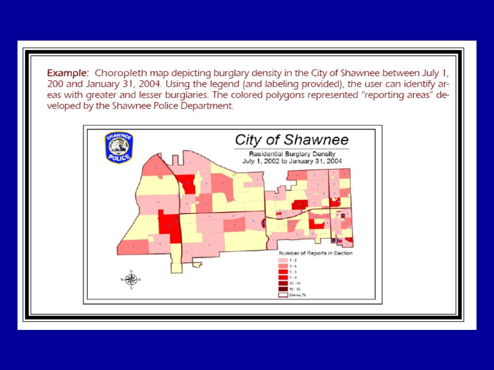
When incidents are geocoded, a list or database of crimes is turned into a map of those crimes This map can now tell a story about the police data Thematic maps are created Point Symbol maps Choropleth maps Graduated Symbol maps

Why map crime? Identify patterns and problems Identify hot spots Use as a visual aid Shows relationship between geography & other factors Look at direction of movement Query data Track changes in crime Make maps for police deployment …And many other reasons

After you create the map, then analyze Why? To answer questions about data Historically, analysts relied heavily on visual interpretation of the map to answer the questions To identify hot spots To draw conclusions To recommend responses

Why is visual interpretation not always possible? Can’t easily pick out hot spots among 1000s of data points Can’t detect subtle shifts in the geography of a crime pattern over time Can’t calculate correlations between two (or more) geographic variables Can’t analyze travel times among complex road networks Can’t apply complicated journey-to-crime calculations across tens of 1000s of grid cells Spatial Statistics…a need filled by CrimeStat

CrimeStat III First released in August, 1999
Current version, 3.1, released March 2007 Not a GIS & does not create or display maps It reads the files geocoded by a GIS and then exports the results into formats the GIS can read Effective use of CrimeStat requires a GIS and knowledge of its use

CrimeStat III With geocoded crime data, CrimeStat can perform calculations and output map layers including (but not limited to): Mean/center of minimum distance of a group of incidents An area representing the standard deviation of a group of incidents or the entire geographical extent of a group of incidents Statistics measuring the spatial relationship between points (con’t next slide)

CrimeStat III (con’t) Statistics that measure the level of clustering or dispersion within a group of incidents Distance measurements between points Identification of hot spots based on spatial proximity Estimation of density across a geographic area through “kernel smoothing” Statistics that analyze the relationship between space and time (con’t next slide)

CrimeStat III (con’t) Statistics that analyzed the movement of a serial offender Routines that estimate the likelihood that a serial offender lives at any location in the region, based on journey-to-crime research …And much, much more….

CrimeStat III Using CrimeStat statistical routines, an analyst is able to Identify crime patterns & series Identify the ‘target area’ in which a serial offender is most likely to strike next Identify and triage hot spots Conduct a risk analysis across a jurisdiction based on known crime locations Create a ‘geographic profile’ to assist in investigating suspected offenders Optimize patrol routes and response times

CrimeStat III CrimeStat is valuable for Tactical Crime Analysis
Crime Patterns, Crime Series, Forecasting Strategic Crime Analysis Hot Spots, Problem Solving, Geographic Profiling Operations Analysis Patrol Routes, Patrol Districts, Response Times

Spatial Statistics in Crime Analysis
Some maps are simplistic and require only a simple scanning and a limited amount of human perception Hot Spot Identification, Spatial Forecasting

Some map interpretation are impossible without spatial statistics Geographic Profiling, Density Mapping

It would be difficult to see subtle shifts in crime incidents (within a series or pattern or over years of changes in geography within a jurisdiction) These incidents are actually moving northwestward over time…..

Other spatial statistics tools available to crime analysts Those that come with ArcView & MapInfo ArcView’s SpatialAnalyst ArcView’s Animal Movements extension Geographic Profiling software Rigel byECRI Dragnet from Center for Investigative Psychology SPSS Microsoft Excel CrimeStat puts all of the methods into one application…and it’s free!

Hardware and Software Windows operating system Must have 256 MB of RAM
Windows 2000, Windows XP and Vista Must have 256 MB of RAM Must have 800MHz processor speed Best is 1GB of Ram / 1.6MHz processor Need a GIS to display the CrimeStat outputs (ArcMap used in workbook)

Notes About the Book & Course
Introductory course only Certain routines/techniques most applicable to crime analysts So much more to learn… Correlated Walk Analysis Journey-to-Crime Crime Travel Demand Basic GIS background required

Exploring Lincoln, NE Lessons & screen shots use data from Lincoln
Some data has been manipulated or even created/invented for lessons Outputs / maps should not be taken as an accurate representation of crime in Lincoln Before starting the CrimeStat lessons, explore the Lincoln data in the GIS

Exploring Lincoln, NE Open your GIS Add the following data layers
Streets Citylimit Cityext Streams Waterways Display in a logical order Apply styles and labels as you please

Exploring CrimeStat There are five tab across the “top” of the CrimeStat screen Under each tab, additional tabs appear They are color coordinated (in case you lose your place) The five main tabs are: Data Setup - Spatial Description Spatial modeling - Crime travel demand Options

Data Setup In CrimeStat
Screen you specify the files on which you want CrimeStat to perform The calculations The various parameters Note: CrimeStat does not query data You must already have the data queried out CrimeStat will perform spatial calculations on the entire file

Data Setup CrimeStat requires at least one primary file which will likely contain your crime data Allows for a secondary file for comparisons in some types of spatial statistics Like comparing homicides (primary file) to poverty rates (secondary file) A reference file is either imported or created in CrimeStat A measurement parameters tab is provided to input geographic information on your jurisdiction, the length of the street network and the methods for calculating distance.

Spatial Description Like descriptive statistics-analyze the data “as is” The Spatial Distribution tab includes functions that tell us the central tendency and variance in our data Includes the mean center, standard deviation ellipses and convex hulls The Distance Analysis I screen has functions to measure distances between points Nearest Neighbor Analysis & Ripley’s K help determine the significant of the clustering or dispersion of the incidents Assign primary points to secondary points takes the points from one file and connect them to their nearest neighbor in another file

Spatial Description Distance Analysis II has functions that create matrices of distances between points Hot Spot Analysis I and II contains a series of routines that help us identify, flag, and triage clusters in our incident data

Spatial Modeling Helps create interpolations & predictions based on our data The Interpolation tab contains the options to create a kernel density estimation resulting in a density map. Space-time analysis is about analyzing progression in a series of crimes, including the moving average (covered) and correlated walk analysis (not covered) Journey-to-Crime and Bayesian Journey-to-Crime Estimation helps determine the likelihood of a serial offender living in a certain area based on the locations of his offenses (not covered)

Crime Travel Demand Helps analyze travel patterns of offenders over large metropolitan areas Emerging and potentially valuable analysis Very complex Not included in this workbook

Summary of CrimeStat Functions
Refer to Table 1-1, pages 12-13 Note the functions included in the workbook Chapter 3 Mean Center, Standard Deviation Ellipse, Median Center, Center of Minimum Distance, Convex Hull Chapter 4 Nearest Neighbor Analysis, Assign primary points to secondary points Chapter 5 Mode (Hot Spot), Fuzzy Mode, Nearest Neighbor Hierarchical Spatial Clustering, Spatial and Temporal Analysis of Crime Chapter 6 Kernel Density Estimate Chapter 7 Spatial-Temporal Moving Average

Chapter Two Getting Data into (and out of) CrimeStat

In Chapter Two... File formats understood by CrimeStat
Projection and coordinate system considerations Associating your data with values needed by CrimeStat Accounting for missing values Creating a reference grid Measurement parameters Getting data out of CrimeStat

Introduction Data must already be created, queried and geocoded
If your RMS or CAD automatically assigns geographic coordinates, you can import the data without going thru a GIS first CrimeStat can read many formats, including .txt., .dat, .dbf, .shp, .mdb and ODBC data sources

Introduction No matter the format, for CrimeStat to analyze the data, the attribute table must contain X and Y coordinates X and Y coordinates: X coordinate value denotes a location that is relative to a point of reference to the east or west and the Y coordinate to the north or south Exception: ArcGIS ‘shapefiles’ which CrimeStat will interpret automatically and add the X and Y coordinates as the first columns in the table

Introduction Coordinate Systems
Longitude (X) and Latitude (Y) data (spherical coordinates) Can be determined easily because the X coordinate will be a negative number (well, in North and South America) If data is in this format, CrimeStat doesn’t need anything else CrimeStat only reads long/lat data in decimal degrees (used by most systems) U.S. State Plane Coordinates, North American Datum of 1983 (projected coordinates) Specific to each state; based on an arbitrary reference point to the south and west of the state’ boundaries. CrimeStat needs to know measurement units (feet/meters)

Entering Your First Primary File
Open basemap in ArcView Add burglary series shapefile Check projection and coordinate system Launch CrimeStat Add shapefile to CrimeStat Direct CrimeStat to X and Y coordinates Select coordinate system and data units

Other Settings and Options
These are not required Intensity – tells CrimeStat how many times to ‘count’ each point. Default is to count each point once Weight allows us to apply different statistical calculations to different points Rarely used; but will see in a future chapter Time is used in several CrimeStat space-time calculations Must be input as integers or decimal numbers; will see in a future chapter

The missing value column allows us to account for bad data Tell CrimeStat which records to ignore when performing calculations Default is ‘blank’ which excludes blank fields and those with nonnumeric values Users often choose “0” Enter each missing value (-1, 99, 999) Cannot enter ranges

Directional and distance fields are used if your data uses polar coordinate systems This is rare The secondary file screen allows us to enter a second file to relate to the first Must use the same coordinate system and data units as the primary files Cannot include a time variable

Creating a Reference Grid
CrimeStat needs to know the extent of the jurisdiction The reference file is a grid that sits over the entire study area Can be imported or created by CrimeStat To have CrimeStat create the grid Specify coordinates of lower left and upper right extremities of the jurisdiction Coordinates must be in the same system as the primary file

Creating a Reference Grid
Select the Reference File tab; create grid Enter values for Lower Left & Upper Right Specify grid parameters Either distance for each cell, or Number of columns desired Save ‘LincolnGrid’

Measurement Parameters
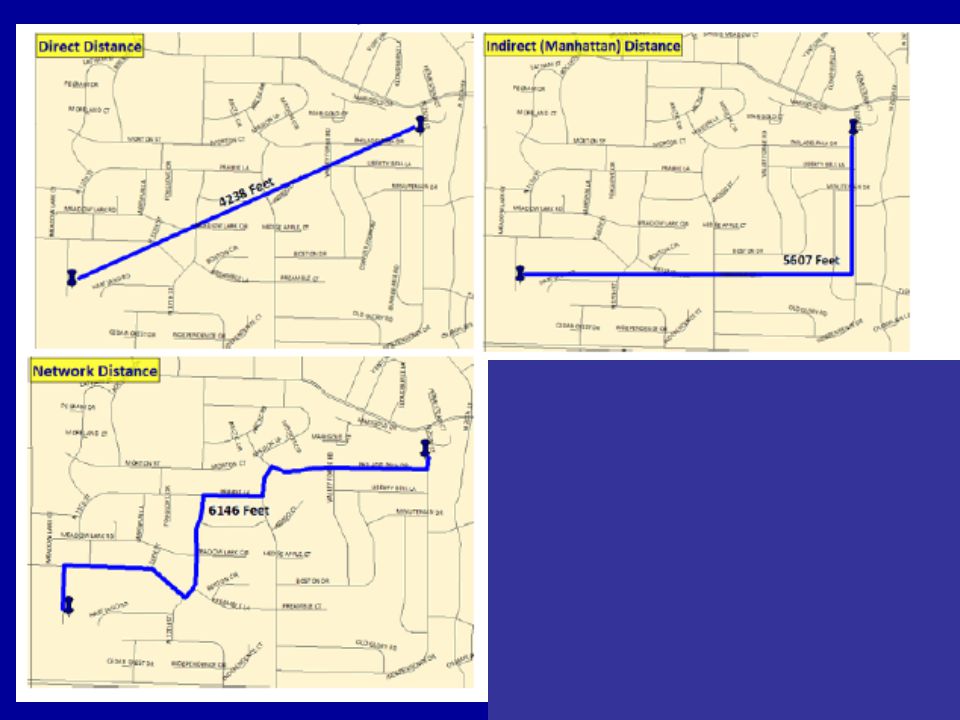
Final bits of data for certain routines Total area of jurisdiction (88.19 square miles in Lincoln) Length of street network is the sum of all of the individual lengths of the streets ( miles in Lincoln) The distance measurement tells CrimeStat how we want to see the distances calculated Direct (as the crow flies), Indirect or Manhattan (along a grid) or Network (uses actual road network)

Entering Measurement Parameters
Select the Measurement Parameters tab Enter values for Area & Length of street Network Choose “Indirect (Manhattan)” for type of distance measurement 49

Getting Data Out of CrimeStat
If the routine results in calculations for a number of records, it exports as a .dbf If the routine results in one or more sets of coordinates, exports as a .shp for ArcView a .mif for MapInfo a .bna for Atlas GIS boundary file

Chapter Three Spatial Distribution

In Chapter Three... Spatial Forecasting Mean and median centerpoints
Measures of variance Analyzing a cluster Limitations of spatial distributions

Introduction Introducing Spatial Distribution
Forecasting Part Art / Part Science Probability Of being right Of being wrong Forecasting is inherent in any spatial or temporal analysis

Spatial Forecasting Two Step Process
Identify the target area for the next incident Identify potential targets in the target area

Spatial Forecasting Targets
Consider availability of targets in any given area Banks, restaurants, convenience stores (vs.) Pedestrians, parked cars, houses 57

Spatial Forecasting Three types of spatial patterns in tactical crime analysis Those that cluster Concentrated in an area, but randomly dispersed Those that walk Offender moving in a predictable manner in distance & direction Hybrids Multiple clusters with predictable walks, or Cluster in which the average points “walks”

Types of Spatial Patterns in Tactical Analysis

Spatial Distribution How are the crimes distributed?
Average location? Greatest volume / concentration? Boundaries? Questions can be answered by looking at (points): Mean Center - Geometric Mean Harmonic Mean - Median Center Center of Minimum Distance

Spatial Distribution Questions can be answered by looking at (areas):
Standard Deviation of X & Y Coordinates Standard Distance Deviation Standard Deviation Ellipse Two Standard Deviation Ellipse

Measures of Spatial Distribution
Mean Center Intersection of the mean of the X coordinates and the mean of the Y coordinates Mean Center of Minimum Distance The points at which the sum of the distance to all the other points is the smallest Median Center Intersection between the median of the X coordinates and the median of the Y coordinates Great if you have outliers! 62

Measures of Spatial Distribution
Geometric Mean & Harmonic Mean Alternate measures of the mean center Just rely on the mean 63

Measures of Concentration
Standard Deviation of the X and Y coordinates A rectangle encloses the area in which four lines intersect: one s/d above the mean of the X axis, one s/d below the mean on the X axis, one s/d above the mean on the Y axis and one s/d below the mean on the Y axis Standard Distance Deviation Calculates the linear distance from each point to the mean center point, then draws a circle around one s/d from the center point. 64

Measures of Concentration
Standard Deviational Ellipse Similar to the standard distance deviation but accounts for skewed distributions, minimizing any “extra space” that might appear in a circle Convex Hull Polygon Encloses the outer reaches of the series. No points fall outside of the polygon Outliers may greatly increase the size of the polygon 65

Analyzing a Cluster Open burglary series in ArcView
Click on Spatial Description tab in CrimeStat Select appropriate checkboxes Save results for “burglaryseries” Compute Ten (10) ArcView shapefiles will be created Open each, format and compare 66

Exercises – Page 33 & 34 67

Cautions & Caveats You generally can’t do this by hand
Wouldn’t account for multiple incidents at a single location Larger series or large volumes of crime would be nearly impossible to interpret on your own CrimeStat can be precise; you cannot (usually) Nothing should replace your experience, intuition and the obvious (see Figure 3-7) 68

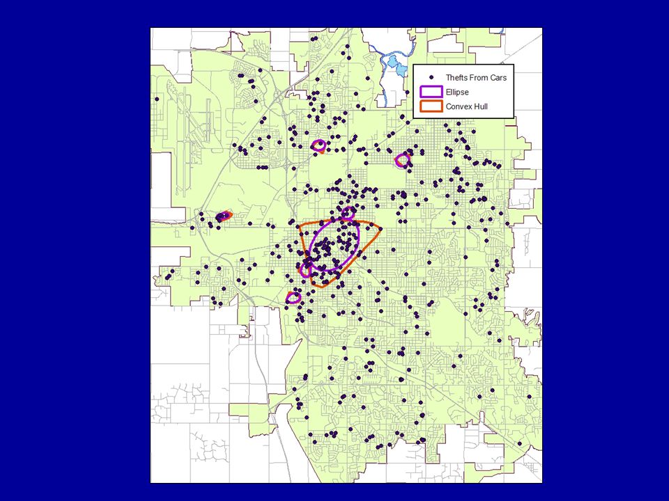
Figure 3-7: An unhelpful spatial distribution
Figure 3-7: An unhelpful spatial distribution. The mean center, standard deviation ellipse, and standard distance deviation circle are technically correct, but they miss the point of the pattern, which is that it appears in two clusters. The analyst in this case would probably want to create a separate dataset for each cluster and calculate the spatial distribution on them separately.

Chapter Four Distance Analysis

In Chapter Four... Nearest neighbor analysis
Comparing relative clustering and dispersion for multiple offense types Assigning points from one dataset to their nearest neighbor in another dataset

Introduction Distance Analysis – statistics for describing properties of distances between incidents including nearest neighbor analysis, linear nearest neighbor analysis and Ripley’s K statistic Answers questions about the dispersion of incidents Answers questions to help us identify where crimes concentrate 72

Nearest Neighbor Analysis
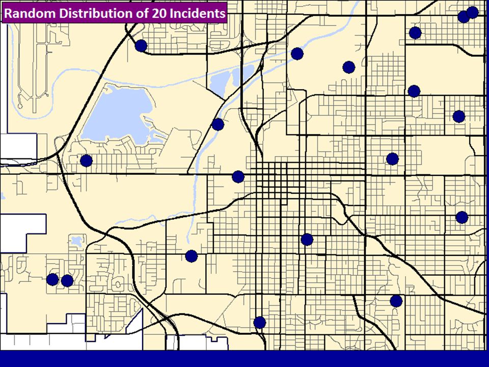
With random crimes scattered in a jurisdiction, it’s normal to have small cluster and wide gaps, but you’d still have an average distance CrimeStat compares the actual average distance between points and their nearest neighbors with what would be “expected” in a random distribution Now you can identify if your incidents are significantly clustered or dispersed. 73

Measures for Distance Analysis
Two primary measures for distance analysis in CrimeStat Nearest neighbor analysis Ripley’s K statistic (not covered in this workbook) 74

Measures the distance of each points to its nearest neighbor, determines the mean distances between neighbors and compared the mean distance to what would have been expected in a random distribution Can run routine to nearest, second nearest, third, etc. User define whether distance is Direct (standard) Indirect (linear) Based on a Network 77

NNA produces the Nearest Neighbor Index (NNI) Score of 1 = no discrepancy between expected distance and measured distance Score lower than 1 = incidents are more clustered than would be expected Scores higher than 2 = incidents are more dispersed than would be expected 78

Most crime types show clustering Geography plays a significant role No business burglaries in places without businesses No residential burglaries in places without residences No bank robberies in cities with no banks Primary value for analysts Conduct distance analysis for several crimes and compare the results to each other You can then determine which offenses are most clustered into “hot spot” and which are more disperse 79

Comparing Distances for Three Offenses
Set up data in new CrimeStat session On Measurement Parameters, enter jurisdiction information and type of distance measurement Check Nearest Neighbor Analysis box on Spatial description/Distance Analysis I tab Compute and examine results Repeat for other files Examine findings 80

Residential Burglaries
Crime Actual Expected NNI Robberies Residential Burglaries Thefts from Autos

Cautions, Caveats and Notes
We are computing single nearest neighbor You can change to another value, but not higher than 100 Significance is only calculated on single nearest Limited utility for doing this Nearest Neighbors may occur on borders NNA overestimates in this case, compensating for the “edge effect” if “Border correction” option is chosen 82

Assigning Primary Points to Secondary Points
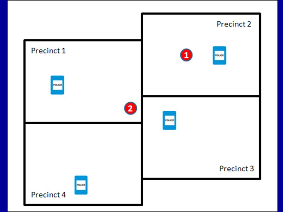
Two ways to conduct Nearest Neighbor Assignment Assigns each point in the primary file to the nearest point in the secondary file Point-in-polygon Assignment CrimeStat interprets the geography of a polygon rile (like police beats) and calculates how many points fall within each file, regardless of anything a point is technically closest to ArcGIS & MapInfo can perform this easily 83

Assigning Primary Points to Secondary Points
Set up CrimeStat for “afternoonhousebreaks” Add schools on the Secondary File tab On Spatial Description / Distance Analysis I tab, check Assign Primary Points to Secondary Points box Save results Compute and examine results 85

Chapter Five Hot Spot Analysis

In Chapter Five... Summary of different hot spot routines
Mode and fuzzy mode Nearest neighbor hierarchical spatial clustering Spatial and Temporal Analysis of Crime

Introduction Identifying hot spots
A spatial concentration of crime, or A geographic area representing a small percentage of the study area which contains a high percentage of the studied phenomenon Can be on a variety of scales A hot address A hot office building A hot block A hot area 88

Hot Spot Routines Mode Fuzzy Mode
Identifies the geographic coordinates with the highest number of incidents Fuzzy Mode Identifies the geographic coordinates, plus a user-specified surrounding radius, with the highest number of incidents Nearest-Neighbor Hierarchical Spatial Clustering Builds on NNA by identifying clusters of incidents 89

Hot Spot Routines Spatial & Temporal Analysis of Crime (STAC)
Alternate means of identifying clusters by “scanning” the point and overlaying circles on the map until the density concentrations are identified K-Means Clustering User specifies the number of clusters and CrimeStat positions them based on the density of incidents 90

Hot Spot Routines Aneslin’s Local Moran statistic
Compares geographic zones to their larger neighborhoods and identifies those that are unusually high or low Kernel Density Interpolation A spatial modeling technique 91

Mode Just counts the number of incidents at one spot
Note: same address vs. X & Y coordinates Which is your records management or CAD system receiving? How would this effect the mode? 92

Mode Set up a new CrimeStat session
Check Mode on Spatial description / Hot Spot Analysis I tab Click compute Top 45 locations, ordered by frequency Save result to (.dbf) (You could then import to GIS) 93

Fuzzy Mode User can specify a search radius around each point
Hence, it will include all of the points within that radius in the count For agencies with GPS data, may be only way to find hot spots Unlikely two incidents will have identical X & Y coordinates 94

Figures 5-3 and 5-4: Accidents at several intersections
Figures 5-3 and 5-4: Accidents at several intersections. The agency has been ultra-accurate in its geocoding, assigning the accidents to the specific points at the intersections where they occur. The mode method (left) would therefore count each point only once, whereas the fuzzy mode method (right) aggregates them based on user-specified radiuses

Fuzzy Mode Return to CrimeStat screen Uncheck Mode / Check Fuzzy Mode
Search radius of 500 feet Save result to Compute Note different results from Mode Create proportional symbol map based on frequency in ArcView 96

Nearest Neighbor Hierarchical Spatial Clustering
Builds on NNA (NNA determines if a particular crime was more clustered than might be expected by random chance) NNH takes the analysis to the next level by actually identifying those clusters CrimeStat clusters groups of pairs that are unusually close together It creates “first order”, “second order” etc. clusters Continues until it cannot locate any more clusters Creates both s/d ellipses & convex hulls 97

Options that can be used when running NNH Fixed distance vs. threshold distance Becomes a subjective measure vs. probability Minimum points per cluster Default is 10 Alter depending on volume & type of crime Search Radius Bar Adjust threshold distance and associated probability Left – smallest distance, but % confidence Right – greatest distances, but only .1% confidence 98

Options (con’t) Number of standard deviations for the ellipses Single s/d is the default/norm Can make small ellipses that are hard to view at a small scale Another option is two s/d’s May exaggerate the size of the hot spot Convex hull vs. ellipse Convex hull has greater accuracy Convex hull has a higher density than an ellipse Convex hulls are defined by the data 99

Data Setup; Measurement parameters Spatial description, Hot Spot Analysis I, uncheck Fuzzy Mode, check NNH Adjust minimum number points & size of ellipses Save ellipses to…. Save convex hulls to…. Compute Add to ArcView project; evaluate Experiment with other NNH settings 100

Spatial and Temporal Analysis of Crime (STAC)
Originally a separate program; integrated into CrimeStat in Version 2 Produces ellipses and convex hulls STAC’s algorithm scans the data by overlaying a grid on the study area and applying a search circle to each node of the grid Size is specified by user Routine counts the number of points in each circle to identify the densest clusters 102

Spatial and Temporal Analysis of Crime (STAC)
Un-check NNH option; check STAC option Set STAC Parameters Note reference file “From data set” option Save ellipses to…. Save convex hulls to…. Compute Open in ArcView Examine results Run with other parameters 103

Final Notes on Hot Spot Identification
Clusters are identified based on volume, not risk Two areas of town 3 burglaries in rural area vs. 20 burglaries in midtown Technique to normalize hot spots available Risk-Adjusted Nearest Neighbor Hierarchical Spatial Clustering (RNNH) Relies on a secondary file with a denominator Number of houses, parking spots, etc In all of these routines, subjectivity plays a role 105

Chapter Six Kernel Density Estimation

In Chapter Six... How kernel density estimation works
Understanding different interpolation methods Guidelines for kernel size and bandwidth Creating and mapping a kernel density estimation Uses and misuses of kernel density

Introduction Crime Analysts most often create Pin maps
Kernel density maps AKA surface density maps AKA continuous surface maps AKA density maps AKA isopleth maps AKA grid maps AKA hot spot maps 108

Introduction Kernel Density Estimation (KDE)
Generalizes data over larger regions As opposed to volumes of incidents at specific locations Good image to show estimation Comparative to weather maps “What is going on here is probably going on there” Question on accuracy in crime analysis Provides a “risk surface” more than an actual picture of what “is” occurring 109

How KDE Works Every point on the map has a density estimate based on its proximity to crime incidents Done by overlaying a grid on top of the map Calculates the density estimate for the centerpoint of each grid cell Number of cells in the grid is defined by the user 110

How KDE Works CrimeStat measures the distance between each grid cell centerpoint and each incident data point and determines the cell weight for that point Sums the weights received from all points into the density estimate But the weight of each cell depends on three things…. 111 111

How KDE Works Weight of each cell depends on
Distance from the grid cell centerpoint to the incident data point Size of the radius around each incident data point Method of interpolation 112

How KDE Works Method of Interpolation
KDE places a symmetrical surface called a kernel over each point (size specified by user, shape specified by method of interpolation) the value is then smoothed throughout the kernel finally, overlay a grid 113 113

How KDE Works In a map, the grid cells are color-coded based on the density Often reds for hottest area and blues for coolest

KDE Parameters Many parameters involved
Analyst must use experience & judgment Single versus dual kernel density estimates Single is usually used in crime analysis Dual can help normalize data for population or other risk factors or calculate change from one time to the next Bandwidth Refers to the size of the cone; specified by user 115

KDE Parameters Methods of interpolation (shape of bandwidth)
Normal (bell curve) peaks & declines rapidly No defined radius; continues across entire grid 116

Uniform (flat) distribution Represented by cylinder; all points in radius equal 117 117

Quartic (spherical) distribution Gradual curve; density highest over point; falls to limit of radius 118 118

KDE Parameters Methods of interpolation (con’t)
Triangular (conical) distribution Peaks above the point; falls off in a linear manner to edges of radius 119 119

KDE Parameters Methods of interpolation (con’t)
Negative exponential distribution Curve that falls off rapidly from the peak to a specified radius 120

KDE Parameters Each method will produce different results
Triangular & negative exponential produce many small hot and cold spots Quartile, uniform and normal distribution functions smooth data more Negative exponential Normal Distribution 121

KDE Parameters Parameter to specify size of bandwidth
Choice of Bandwidth Minimum Sample Size Interval With “adaptive”, CrimeStat will adjust the size of the kernal until it’s large enough to contain the minimum sample size With “fixed interval” bandwidth, you specify the size 122

KDE Parameters Output units (any will work fine) Absolute densities
Sum of all the weights received by each cell, but re-scaled so the sum of the densities equal the total number of incidents (default) Relative densities Divides the absolute densities by the area of the grid “Red represents “X” points per square mile, not per grid cell” Probabilities Divides the density by the total number of incident “Chance” that any incident occurred in that cell 123

KDE Parameters Deciding which parameters to use for a particular dataset Across how great an area is this incident likely to have an effect Adjust interval distance (bandwidth size) How much of this effect should remain at the original location; how much dispersed? Adjust method of interpolation 124

Incident Type Interval Interpolation Method Reasoning Residential burglaries 1 mile Moderately dispersed: quartic or uniform Some burglars choose particular houses, but most cruise neighborhoods looking for likely targets. A housebreak in any part of a neighborhood transfers risk to the rest of the neighborhood. Domestic violence 0.1 mile Tightly focused: negative exponential Domestic violence occurs among specific individuals and families. Incidents at one location do not have much chance of being contagious in the surrounding area. Commercial robberies 2 miles Focused: triangular or negative exponential A commercial robber probably chooses to strike in a commercial area, and then looks for preferred targets (banks, convenience stores) within that area. The wide area may thus be at some risk, but the brunt of the weight should remain with the particular target that has already been struck. Thefts from vehicles 0.25 mile Dispersed: uniform If a parking lot experiences a lot of thefts from vehicles, your GIS will probably geocode them at the center of the parcel. This method ensures that the risk disperses evenly across the parcel and part of the surrounding area (which probably makes sense)—but not too far, since we know that parking lots tend to be hot spots for specific reasons.

Creating a KDE Data setup; add ArcView SHP file theftfromautos;
Create reference grid on Reference File tab On Spatial modeling tab, Interpolation sub-tab, chose Single KDE; adjust bandwidth and select interpolation method Save result to; compute Open KLFA shapefile in ArcView and create a choropleth map Experiment with different settings 126

Dual KDE KDE based on two files Primary & Secondary
Primary use is to normalize for risk In single KDE, hot spots are based on volume In dual KDE, hot spots are based on risk Four things to keep in mind Sometimes you just want volume Data for secondary file is hard to come by The point data in the secondary file is interpolated just like the primary file You cannot use a different interpolation method for numerator and denominator (but you can use an adaptive bandwidth) 127

Dual KDE Set up Secondary File like Primary File except
Ratio of Densities Divides the density in the primary file with the density in secondary file Log ratio of densities Helps control extreme highs and lows Valuable in strongly skewed distributions Absolute difference in densities Subtracts the secondary file densities from the primary file densities Valuable in analyzing one time period to the next 128

Dual KDE Set up Secondary File like Primary File except (con’t)
Relative difference in densities Option divides primary and second files densities by area of the cells before subtracting them (just like absolute difference) Sum of densities Adds two densities together Useful to show combined effects of two types of crime Relative sum of densities Divides primary and second files by the area of the cells before adding them 129

Dual KDE On Data Setup, remove larcey from autos and add resburglaries.shp file On Secondary File, select censusblocks.dbf, set variables, including Z (Intensity) On Spatial Modeling, Interpolation tabs, select “Dual” box (check weighting variable option) Save Result to (.shp) Open ArcView, add layer, create choropleth map 130

Dual KDE Uses and Cautions
KDE is a hot spot technique, but it is part theoretical KDE maps are interpolations Meaning incidents did not occur at all of the locations within the hottest color Creates a uniform risk surface (which is rare) You can only have bank robberies where there are banks Hence, interpret a KDE in reference to where suitable targets may exist within the risk surface 131

Chapter Seven Spatial Temporal Moving Average

In Chapter Seven... Understanding the Spatial Temporal Moving Average
Using a time variable in CrimeStat

Introduction Spatial-Temporal Moving Average (STMA)
Set of points in robbery series But mean, SD, SDE doesn’t represent the series Something is “off” Recall two types of crime patterns (Chpt 3) Those that cluster Those that walk 134

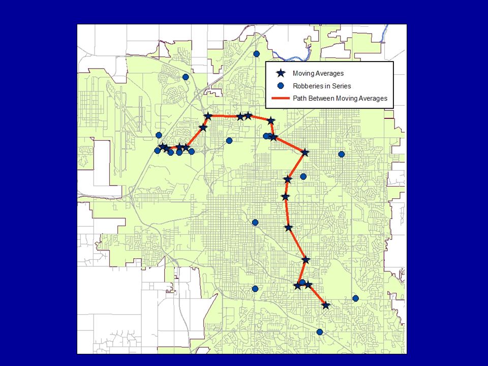
Introduction This one walks

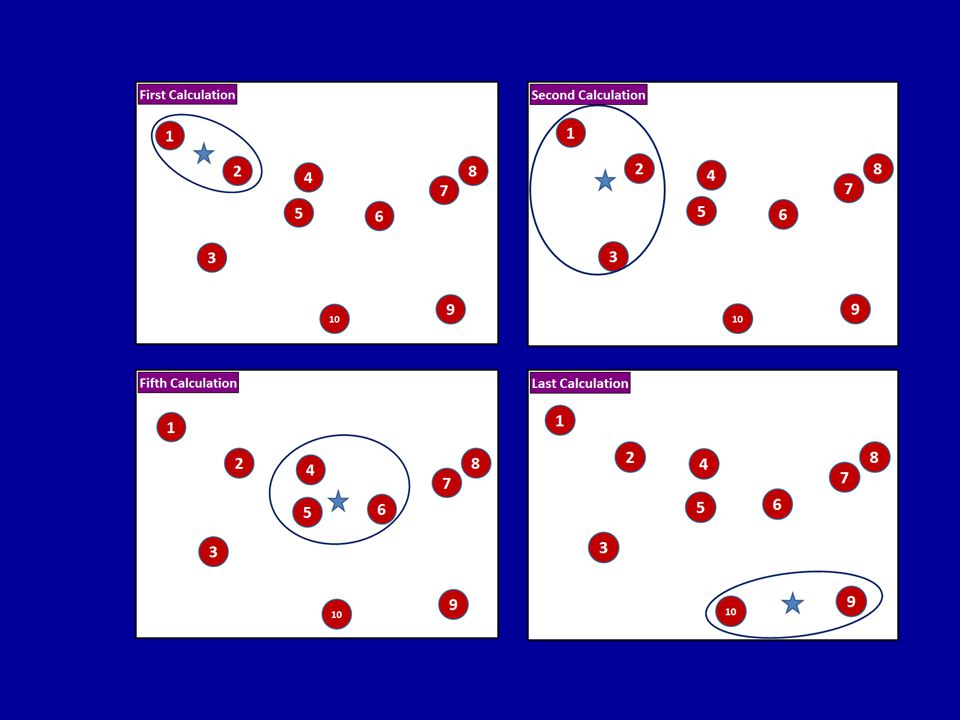
Introduction STMA calculates the mean center at each point in the series Tracks how it moves over time User specific how many point are included in each calculation using the “span” parameter A span of “3” means it calculates the average for that point and the two points on either side of it in the sequence Final result is a series of moving average points tied together to create a path 136

Introduction Span is the only parameter in the STMA calculation
Use an odd number for the center observation to fall on an actual incident Default is five (5) Use caution when changing it Too high – won’t see much movement Too low – just viewing changes from one incident to the next 139

Introduction All of the “Space-Time” analysis routines require a time variable STMA needs it so it will know how the incidents are sequenced. CrimeStat will not accurately calculate actual date/time fields like “06/09/2008” or “15:10.” Instead, it requires actual numbers. It doesn’t matter where the numbers start as long as the intervals are accurate, so if your data goes from June 1, 2008 to July 15, 2008, you could assign “1” for June 1, “2” for June 2, “31” for July 1,” and so on—or you could assign “3000” for June 1 and “3031” for July 1. It’s really only the intervals that matter.

Introduction Microsoft makes date/time conversions easy
It stores dates as the number of days elapsed since January 1, 1900 and times as proportions of a 24-hour day In either Access or Excel, we can convert date values to these underlying numbers, so June 1, 2008 becomes 39600, and 15:10 becomes We have already used Excel to figure the Microsoft date from the actual date, and the field is labeled “MSDate”

STMA New CrimeStat session using CSRobSeries.shp file
Add “Time” setting Note it needs a number, not an actual date/time Already calculated in MSExcel; use MSDate Time Unit = Days Spatial Modeling, space-time analysis tab, check STMA 142

STMA Save Output as .dbf Save Graph as ArcView SHP Compute
CSRobSeries Save Graph as ArcView SHP Compute Examine results Offender moving which way? What targets are available? Forecast next offense 143

CrimeStat III

Susan C. Smith Christopher W. Bruce

Similar presentations

Presentation on theme: "Susan C. Smith Christopher W. Bruce"— Presentation transcript:

Similar presentations

About project

Feedback

Log in

Auth with social network:

Susan C. Smith Christopher W. Bruce

Similar presentations

Presentation on theme: "Susan C. Smith Christopher W. Bruce"— Presentation transcript:

Similar presentations

About project

Feedback