1. Topics in Microeconometrics William Greene Department of Economics Stern School of Business

2. Part 3: Basic Linear Panel Data Models

5. Cornwell and Rupert Data Cornwell and Rupert Returns to Schooling Data, 595 Individuals, 7 Years Variables in the file are EXP = work experience WKS = weeks worked OCC = occupation, 1 if blue collar, IND = 1 if manufacturing industry SOUTH = 1 if resides in south SMSA= 1 if resides in a city (SMSA) MS = 1 if married FEM = 1 if female UNION = 1 if wage set by union contract ED = years of education BLK = 1 if individual is black LWAGE = log of wage = dependent variable in regressions These data were analyzed in Cornwell, C. and Rupert, P., "Efficient Estimation with Panel Data: An Empirical Comparison of Instrumental Variable Estimators," Journal of Applied Econometrics, 3, 1988, pp. 149-155. See Baltagi, page 122 for further analysis. The data were downloaded from the website for Baltagi's text.

7. Balanced and Unbalanced Panels Distinction: Balanced vs. Unbalanced Panels A notation to help with mechanics z i,t, i = 1,…,N; t = 1,…,T i The role of the assumption Mathematical and notational convenience: Balanced, n=NT Unbalanced: Is the fixed T i assumption ever necessary? Almost never. Is unbalancedness due to nonrandom attrition from an otherwise balanced panel? This would require special considerations.

8. Application: Health Care Usage German Health Care Usage Data, 7,293 Individuals, Varying Numbers of Periods This is an unbalanced panel with 7,293 individuals. There are altogether 27,326 observations. The number of observations ranges from 1 to 7. (Frequencies are: 1=1525, 2=2158, 3=825, 4=926, 5=1051, 6=1000, 7=987). (Downloaded from the JAE Archive) Variables in the file are DOCTOR = 1(Number of doctor visits > 0) HOSPITAL= 1(Number of hospital visits > 0) HSAT = health satisfaction, coded 0 (low) - 10 (high) DOCVIS = number of doctor visits in last three months HOSPVIS = number of hospital visits in last calendar year PUBLIC = insured in public health insurance = 1; otherwise = 0 ADDON = insured by add-on insurance = 1; otherswise = 0 HHNINC = household nominal monthly net income in German marks / 10000. (4 observations with income=0 were dropped) HHKIDS = children under age 16 in the household = 1; otherwise = 0 EDUC = years of schooling AGE = age in years MARRIED = marital status

9. An Unbalanced Panel: RWMs GSOEP Data on Health Care N = 7,293 Households

10. Fixed and Random Effects Unobserved individual effects in regression: E[y it | x it, c i ] Notation: Linear specification: Fixed Effects: E[c i | X i ] = g(X i ). Cov[x it,c i ] 0 effects are correlated with included variables. Random Effects: E[c i | X i ] = 0. Cov[x it,c i ] = 0

11. Convenient Notation Fixed Effects – the dummy variable model Random Effects – the error components model Individual specific constant terms. Compound (composed) disturbance

12. Estimating β β is the partial effect of interest Can it be estimated (consistently) in the presence of (unmeasured) c i ? Does pooled least squares work? Strategies for controlling for c i using the sample data

13. The Pooled Regression Presence of omitted effects Potential bias/inconsistency of OLS – depends on fixed or random

14. OLS with Individual Effects

15. Estimating the Sampling Variance of b s 2 (X X) -1 ? Inappropriate because Correlation across observations (Possibly) Heteroscedasticity A robust covariance matrix Robust estimation (in general) The White estimator A Robust estimator for OLS.

16. Cluster Estimator

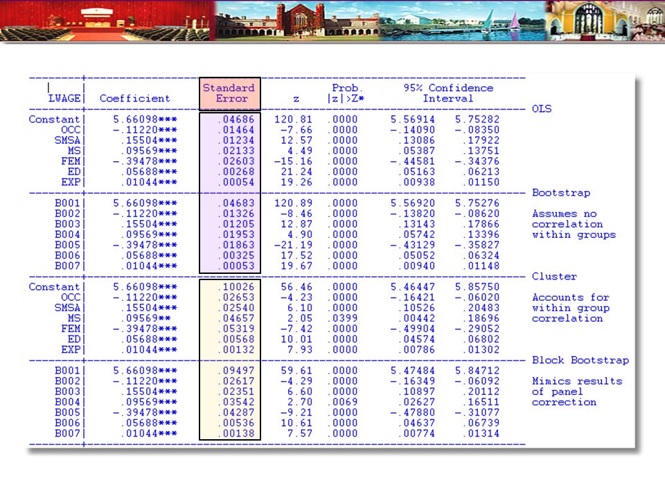
17. Application: Cornwell and Rupert

18. Bootstrap variance for a panel data estimator Panel Bootstrap = Block Bootstrap Data set is N groups of size T i Bootstrap sample is N groups of size T i drawn with replacement.

20. Difference in Differences With two periods, This is a linear regression model. If there are no regressors,

21. Difference-in-Differences Model With two periods and strict exogeneity of D and T, This is a linear regression model. If there are no regressors,

22. Difference in Differences

23. The Fixed Effects Model y i = X i + d i α i + ε i, for each individual E[c i | X i ] = g(X i ); Effects are correlated with included variables. Cov[x it,c i ] 0

24. Estimating the Fixed Effects Model The FEM is a plain vanilla regression model but with many independent variables Least squares is unbiased, consistent, efficient, but inconvenient if N is large.

25. The Within Groups Transformation Removes the Effects

26. Least Squares Dummy Variable Estimator b is obtained by within groups least squares (group mean deviations) a is estimated using the normal equations: DXb+DDa=Dy a = (DD) -1 D(y – Xb)

27. Application Cornwell and Rupert

28. LSDV Results Note huge changes in the coefficients. SMSA and MS change signs. Significance changes completely! Pooled OLS

29. The Effect of the Effects

30. A Caution About Stata and R 2 The coefficient estimates and standard errors are the same. The calculation of the R 2 is different. In the areg procedure, you are estimating coefficients for each of your covariates plus each dummy variable for your groups. In the xtreg, fe procedure the R 2 reported is obtained by only fitting a mean deviated model where the effects of the groups (all of the dummy variables) are assumed to be fixed quantities. So, all of the effects for the groups are simply subtracted out of the model and no attempt is made to quantify their overall effect on the fit of the model. aregxtreg, fe Since the SSE is the same, the R 2 =1SSE/SST is very different. The difference is real in that we are making different assumptions with the two approaches. In the xtreg, fe approach, the effects of the groups are fixed and unestimated quantities are subtracted out of the model before the fit is performed. In the areg approach, the group effects are estimated and affect the total sum of squares of the model under consideration. For the FE model above, R 2 = 0.90542 R 2 = 0.65142

31. Examining the Effects with a KDE Mean = 4.819, Standard deviation = 1.054.

32. Robust Covariance Matrix for LSDV Cluster Estimator for Within Estimator +--------+--------------+----------------+--------+--------+----------+ |Variable| Coefficient | Standard Error |b/St.Er.|P[|Z|>z]| Mean of X| +--------+--------------+----------------+--------+--------+----------+ |OCC | -.02021.01374007 -1.471.1412.5111645| |SMSA | -.04251**.01950085 -2.180.0293.6537815| |MS | -.02946.01913652 -1.540.1236.8144058| |EXP |.09666***.00119162 81.114.0000 19.853782| +--------+------------------------------------------------------------+ +---------------------------------------------------------------------+ | Covariance matrix for the model is adjusted for data clustering. | | Sample of 4165 observations contained 595 clusters defined by | | 7 observations (fixed number) in each cluster. | +---------------------------------------------------------------------+ +--------+--------------+----------------+--------+--------+----------+ |Variable| Coefficient | Standard Error |b/St.Er.|P[|Z|>z]| Mean of X| +--------+--------------+----------------+--------+--------+----------+ |DOCC | -.02021.01982162 -1.020.3078.00000| |DSMSA | -.04251.03091685 -1.375.1692.00000| |DMS | -.02946.02635035 -1.118.2635.00000| |DEXP |.09666***.00176599 54.732.0000.00000| +--------+------------------------------------------------------------+

33. Time Invariant Regressors Time invariant x it is defined as invariant for all i. E.g., sex dummy variable, FEM and ED (education in the Cornwell/Rupert data). If x it,k is invariant for all t, then the group mean deviations are all 0.

34. FE With Time Invariant Variables +----------------------------------------------------+ | There are 3 vars. with no within group variation. | | FEM ED BLK | +----------------------------------------------------+ +--------+--------------+----------------+--------+--------+----------+ |Variable| Coefficient | Standard Error |b/St.Er.|P[|Z|>z]| Mean of X| +--------+--------------+----------------+--------+--------+----------+ EXP |.09671227.00119137 81.177.0000 19.8537815 WKS |.00118483.00060357 1.963.0496 46.8115246 OCC | -.02145609.01375327 -1.560.1187.51116447 SMSA | -.04454343.01946544 -2.288.0221.65378151 FEM |.000000......(Fixed Parameter)....... ED |.000000......(Fixed Parameter)....... BLK |.000000......(Fixed Parameter)....... +--------------------------------------------------------------------+ | Test Statistics for the Classical Model | +--------------------------------------------------------------------+ | Model Log-Likelihood Sum of Squares R-squared | |(1) Constant term only -2688.80597 886.90494.00000 | |(2) Group effects only 27.58464 240.65119.72866 | |(3) X - variables only -1688.12010 548.51596.38154 | |(4) X and group effects 2223.20087 83.85013.90546 | +--------------------------------------------------------------------+

35. Drop The Time Invariant Variables Same Results +--------+--------------+----------------+--------+--------+----------+ |Variable| Coefficient | Standard Error |b/St.Er.|P[|Z|>z]| Mean of X| +--------+--------------+----------------+--------+--------+----------+ EXP |.09671227.00119087 81.211.0000 19.8537815 WKS |.00118483.00060332 1.964.0495 46.8115246 OCC | -.02145609.01374749 -1.561.1186.51116447 SMSA | -.04454343.01945725 -2.289.0221.65378151 +--------------------------------------------------------------------+ | Test Statistics for the Classical Model | +--------------------------------------------------------------------+ | Model Log-Likelihood Sum of Squares R-squared | |(1) Constant term only -2688.80597 886.90494.00000 | |(2) Group effects only 27.58464 240.65119.72866 | |(3) X - variables only -1688.12010 548.51596.38154 | |(4) X and group effects 2223.20087 83.85013.90546 | +--------------------------------------------------------------------+ No change in the sum of squared residuals

36. Fixed Effects Vector Decomposition Efficient Estimation of Time Invariant and Rarely Changing Variables in Finite Sample Panel Analyses with Unit Fixed Effects Thomas Plümper and Vera Troeger Political Analysis, 2007

37. Introduction [T]he FE model … does not allow the estimation of time invariant variables. A second drawback of the FE model … results from its inefficiency in estimating the effect of variables that have very little within variance. This article discusses a remedy to the related problems of estimating time invariant and rarely changing variables in FE models with unit effects

38. The Model

39. Fixed Effects Vector Decomposition Step 1: Compute the fixed effects regression to get the estimated unit effects. We run this FE model with the sole intention to obtain estimates of the unit effects, α i.

40. Step 2 Regress a i on z i and compute residuals

41. Step 3 Regress y it on a constant, X, Z and h using ordinary least squares to estimate α, β, γ, δ.

42. Step 1 (Based on full sample) These 3 variables have no within group variation. FEM ED BLK F.E. estimates are based on a generalized inverse. --------+--------------------------------------------------------- | Standard Prob. Mean LWAGE| Coefficient Error z z>|Z| of X --------+--------------------------------------------------------- EXP|.09663***.00119 81.13.0000 19.8538 WKS|.00114*.00060 1.88.0600 46.8115 OCC| -.02496*.01390 -1.80.0724.51116 IND|.02042.01558 1.31.1899.39544 SOUTH| -.00091.03457 -.03.9791.29028 SMSA| -.04581**.01955 -2.34.0191.65378 UNION|.03411**.01505 2.27.0234.36399 FEM|.000.....(Fixed Parameter)......11261 ED|.000.....(Fixed Parameter)..... 12.8454 BLK|.000.....(Fixed Parameter)......07227 --------+---------------------------------------------------------

43. Step 2 (Based on 595 observations) --------+--------------------------------------------------------- | Standard Prob. Mean UHI| Coefficient Error z z>|Z| of X --------+--------------------------------------------------------- Constant| 2.88090***.07172 40.17.0000 FEM| -.09963**.04842 -2.06.0396.11261 ED|.14616***.00541 27.02.0000 12.8454 BLK| -.27615***.05954 -4.64.0000.07227 --------+---------------------------------------------------------

44. Step 3! --------+--------------------------------------------------------- | Standard Prob. Mean LWAGE| Coefficient Error z z>|Z| of X --------+--------------------------------------------------------- Constant| 2.88090***.03282 87.78.0000 EXP|.09663***.00061 157.53.0000 19.8538 WKS|.00114***.00044 2.58.0098 46.8115 OCC| -.02496***.00601 -4.16.0000.51116 IND|.02042***.00479 4.26.0000.39544 SOUTH| -.00091.00510 -.18.8590.29028 SMSA| -.04581***.00506 -9.06.0000.65378 UNION|.03411***.00521 6.55.0000.36399 FEM| -.09963***.00767 -13.00.0000.11261 ED|.14616***.00122 120.19.0000 12.8454 BLK| -.27615***.00894 -30.90.0000.07227 HI| 1.00000***.00670 149.26.0000 -.103D-13 --------+---------------------------------------------------------

45. The Magic Step 1 Step 2 Step 3

46. What happened here?

47. The Random Effects Model The random effects model c i is uncorrelated with x it for all t; E[c i |X i ] = 0 E[ε it |X i,c i ]=0

48. Error Components Model A Generalized Regression Model

49. Random vs. Fixed Effects Random Effects Small number of parameters Efficient estimation Objectionable orthogonality assumption (c i X i ) Fixed Effects Robust – generally consistent Large number of parameters

50. Ordinary Least Squares Standard results for OLS in a GR model Consistent Unbiased Inefficient True variance of the least squares estimator

51. Estimating the Variance for OLS

52. OLS Results for Cornwell and Rupert +----------------------------------------------------+ | Residuals Sum of squares = 522.2008 | | Standard error of e =.3544712 | | Fit R-squared =.4112099 | | Adjusted R-squared =.4100766 | +----------------------------------------------------+ +---------+--------------+----------------+--------+---------+----------+ |Variable | Coefficient | Standard Error |b/St.Er.|P[|Z|>z] | Mean of X| +---------+--------------+----------------+--------+---------+----------+ Constant 5.40159723.04838934 111.628.0000 EXP.04084968.00218534 18.693.0000 19.8537815 EXPSQ -.00068788.480428D-04 -14.318.0000 514.405042 OCC -.13830480.01480107 -9.344.0000.51116447 SMSA.14856267.01206772 12.311.0000.65378151 MS.06798358.02074599 3.277.0010.81440576 FEM -.40020215.02526118 -15.843.0000.11260504 UNION.09409925.01253203 7.509.0000.36398559 ED.05812166.00260039 22.351.0000 12.8453782

53. Alternative Variance Estimators +---------+--------------+----------------+--------+---------+ |Variable | Coefficient | Standard Error |b/St.Er.|P[|Z|>z] | +---------+--------------+----------------+--------+---------+ Constant 5.40159723.04838934 111.628.0000 EXP.04084968.00218534 18.693.0000 EXPSQ -.00068788.480428D-04 -14.318.0000 OCC -.13830480.01480107 -9.344.0000 SMSA.14856267.01206772 12.311.0000 MS.06798358.02074599 3.277.0010 FEM -.40020215.02526118 -15.843.0000 UNION.09409925.01253203 7.509.0000 ED.05812166.00260039 22.351.0000 Robust – Cluster___________________________________________ Constant 5.40159723.10156038 53.186.0000 EXP.04084968.00432272 9.450.0000 EXPSQ -.00068788.983981D-04 -6.991.0000 OCC -.13830480.02772631 -4.988.0000 SMSA.14856267.02423668 6.130.0000 MS.06798358.04382220 1.551.1208 FEM -.40020215.04961926 -8.065.0000 UNION.09409925.02422669 3.884.0001 ED.05812166.00555697 10.459.0000

54. Generalized Least Squares

55. Estimators for the Variances

56. Practical Problems with FGLS

57. Stata Variance Estimators

58. Application +--------------------------------------------------+ | Random Effects Model: v(i,t) = e(i,t) + u(i) | | Estimates: Var[e] =.231188D-01 | | Var[u] =.102531D+00 | | Corr[v(i,t),v(i,s)] =.816006 | | Variance estimators are based on OLS residuals. | +--------------------------------------------------+ +---------+--------------+----------------+--------+---------+----------+ |Variable | Coefficient | Standard Error |b/St.Er.|P[|Z|>z] | Mean of X| +---------+--------------+----------------+--------+---------+----------+ EXP.08819204.00224823 39.227.0000 19.8537815 EXPSQ -.00076604.496074D-04 -15.442.0000 514.405042 OCC -.04243576.01298466 -3.268.0011.51116447 SMSA -.03404260.01620508 -2.101.0357.65378151 MS -.06708159.01794516 -3.738.0002.81440576 FEM -.34346104.04536453 -7.571.0000.11260504 UNION.05752770.01350031 4.261.0000.36398559 ED.11028379.00510008 21.624.0000 12.8453782 Constant 4.01913257.07724830 52.029.0000 No problems arise in this sample.

59. Testing for Effects: An LM Test

60. Application: Cornwell-Rupert

61. Hausman Test for FE vs. RE EstimatorRandom Effects E[c i |X i ] = 0 Fixed Effects E[c i |X i ] 0 FGLS (Random Effects) Consistent and Efficient Inconsistent LSDV (Fixed Effects) Consistent Inefficient Consistent Possibly Efficient

62. Computing the Hausman Statistic β does not contain the constant term in the preceding.

63. Hausman Test +--------------------------------------------------+ | Random Effects Model: v(i,t) = e(i,t) + u(i) | | Estimates: Var[e] =.235368D-01 | | Var[u] =.110254D+00 | | Corr[v(i,t),v(i,s)] =.824078 | | Lagrange Multiplier Test vs. Model (3) = 3797.07 | | ( 1 df, prob value =.000000) | | (High values of LM favor FEM/REM over CR model.) | | Fixed vs. Random Effects (Hausman) = 2632.34 | | ( 4 df, prob value =.000000) | | (High (low) values of H favor FEM (REM).) | +--------------------------------------------------+

64. Variable Addition

65. A Variable Addition Test Asymptotic equivalent to Hausman Also equivalent to Mundlak formulation In the random effects model, using FGLS Only applies to time varying variables Add expanded group means to the regression (i.e., observation i,t gets same group means for all t. Use Wald test to test for coefficients on means equal to 0. Large chi-squared weighs against random effects specification.

66. Fixed Effects +----------------------------------------------------+ | Panel:Groups Empty 0, Valid data 595 | | Smallest 7, Largest 7 | | Average group size 7.00 | | There are 3 vars. with no within group variation. | | ED BLK FEM | | Look for huge standard errors and fixed parameters.| | F.E. results are based on a generalized inverse. | | They will be highly erratic. (Problematic model.) | | Unable to compute std.errors for dummy var. coeffs.| +----------------------------------------------------+ +--------+--------------+----------------+--------+--------+----------+ |Variable| Coefficient | Standard Error |b/St.Er.|P[|Z|>z]| Mean of X| +--------+--------------+----------------+--------+--------+----------+ |WKS |.00083.00060003 1.381.1672 46.811525| |OCC | -.02157.01379216 -1.564.1178.5111645| |IND |.01888.01545450 1.221.2219.3954382| |SOUTH |.00039.03429053.011.9909.2902761| |SMSA | -.04451**.01939659 -2.295.0217.6537815| |UNION |.03274**.01493217 2.192.0283.3639856| |EXP |.11327***.00247221 45.819.0000 19.853782| |EXPSQ | -.00042***.546283D-04 -7.664.0000 514.40504| |ED |.000......(Fixed Parameter)....... | |BLK |.000......(Fixed Parameter)....... | |FEM |.000......(Fixed Parameter)....... | +--------+------------------------------------------------------------+

67. Random Effects +--------------------------------------------------+ | Random Effects Model: v(i,t) = e(i,t) + u(i) | | Estimates: Var[e] =.235368D-01 | | Var[u] =.110254D+00 | | Corr[v(i,t),v(i,s)] =.824078 | | Lagrange Multiplier Test vs. Model (3) = 3797.07 | | ( 1 df, prob value =.000000) | | (High values of LM favor FEM/REM over CR model.) | +--------------------------------------------------+ +--------+--------------+----------------+--------+--------+----------+ |Variable| Coefficient | Standard Error |b/St.Er.|P[|Z|>z]| Mean of X| +--------+--------------+----------------+--------+--------+----------+ |WKS |.00094.00059308 1.586.1128 46.811525| |OCC | -.04367***.01299206 -3.361.0008.5111645| |IND |.00271.01373256.197.8434.3954382| |SOUTH | -.00664.02246416 -.295.7677.2902761| |SMSA | -.03117*.01615455 -1.930.0536.6537815| |UNION |.05802***.01349982 4.298.0000.3639856| |EXP |.08744***.00224705 38.913.0000 19.853782| |EXPSQ | -.00076***.495876D-04 -15.411.0000 514.40504| |ED |.10724***.00511463 20.967.0000 12.845378| |BLK | -.21178***.05252013 -4.032.0001.0722689| |FEM | -.24786***.04283536 -5.786.0000.1126050| |Constant| 3.97756***.08178139 48.637.0000 | +--------+------------------------------------------------------------+

68. The Hausman Test, by Hand --> matrix; br=b(1:8) ; vr=varb(1:8,1:8)$ --> matrix ; db = bf - br ; dv = vf - vr $ --> matrix ; list ; h =db' db$ Matrix H has 1 rows and 1 columns. 1 +-------------- 1| 2523.64910 --> calc;list;ctb(.95,8)$ +------------------------------------+ | Listed Calculator Results | +------------------------------------+ Result = 15.507313

69. Means Added to REM - Mundlak +--------+--------------+----------------+--------+--------+----------+ |Variable| Coefficient | Standard Error |b/St.Er.|P[|Z|>z]| Mean of X| +--------+--------------+----------------+--------+--------+----------+ |WKS |.00083.00060070 1.380.1677 46.811525| |OCC | -.02157.01380769 -1.562.1182.5111645| |IND |.01888.01547189 1.220.2224.3954382| |SOUTH |.00039.03432914.011.9909.2902761| |SMSA | -.04451**.01941842 -2.292.0219.6537815| |UNION |.03274**.01494898 2.190.0285.3639856| |EXP |.11327***.00247500 45.768.0000 19.853782| |EXPSQ | -.00042***.546898D-04 -7.655.0000 514.40504| |ED |.05199***.00552893 9.404.0000 12.845378| |BLK | -.16983***.04456572 -3.811.0001.0722689| |FEM | -.41306***.03732204 -11.067.0000.1126050| |WKSB |.00863**.00363907 2.371.0177 46.811525| |OCCB | -.14656***.03640885 -4.025.0001.5111645| |INDB |.04142.02976363 1.392.1640.3954382| |SOUTHB | -.05551.04297816 -1.292.1965.2902761| |SMSAB |.21607***.03213205 6.724.0000.6537815| |UNIONB |.08152**.03266438 2.496.0126.3639856| |EXPB | -.08005***.00533603 -15.002.0000 19.853782| |EXPSQB | -.00017.00011763 -1.416.1567 514.40504| |Constant| 5.19036***.20147201 25.762.0000 | +--------+------------------------------------------------------------+

70. Wu (Variable Addition) Test --> matrix ; bm=b(12:19);vm=varb(12:19,12:19)$ --> matrix ; list ; wu = bm' bm $ Matrix WU has 1 rows and 1 columns. 1 +-------------- 1| 3004.38076

71. A Hierarchical Linear Model Interpretation of the FE Model

72. Hierarchical Linear Model as REM +--------------------------------------------------+ | Random Effects Model: v(i,t) = e(i,t) + u(i) | | Estimates: Var[e] =.235368D-01 | | Var[u] =.110254D+00 | | Corr[v(i,t),v(i,s)] =.824078 | | Sigma(u) = 0.3303 | +--------------------------------------------------+ +--------+--------------+----------------+--------+--------+----------+ |Variable| Coefficient | Standard Error |b/St.Er.|P[|Z|>z]| Mean of X| +--------+--------------+----------------+--------+--------+----------+ OCC | -.03908144.01298962 -3.009.0026.51116447 SMSA | -.03881553.01645862 -2.358.0184.65378151 MS | -.06557030.01815465 -3.612.0003.81440576 EXP |.05737298.00088467 64.852.0000 19.8537815 FEM | -.34715010.04681514 -7.415.0000.11260504 ED |.11120152.00525209 21.173.0000 12.8453782 Constant| 4.24669585.07763394 54.702.0000

73. Evolution: Correlated Random Effects

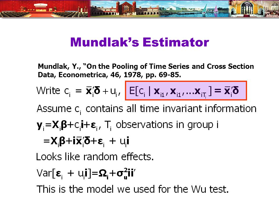
74. Mundlaks Estimator Mundlak, Y., On the Pooling of Time Series and Cross Section Data, Econometrica, 46, 1978, pp. 69-85.

75. Correlated Random Effects

76. Mundlaks Approach for an FE Model with Time Invariant Variables

77. Mundlak Form of FE Model +--------+--------------+----------------+--------+--------+----------+ |Variable| Coefficient | Standard Error |b/St.Er.|P[|Z|>z]| Mean of X| +--------+--------------+----------------+--------+--------+----------+ x(i,t)================================================================= OCC | -.02021384.01375165 -1.470.1416.51116447 SMSA | -.04250645.01951727 -2.178.0294.65378151 MS | -.02946444.01915264 -1.538.1240.81440576 EXP |.09665711.00119262 81.046.0000 19.8537815 z(i)=================================================================== FEM | -.34322129.05725632 -5.994.0000.11260504 ED |.05099781.00575551 8.861.0000 12.8453782 Means of x(i,t) and constant=========================================== Constant| 5.72655261.10300460 55.595.0000 OCCB | -.10850252.03635921 -2.984.0028.51116447 SMSAB |.22934020.03282197 6.987.0000.65378151 MSB |.20453332.05329948 3.837.0001.81440576 EXPB | -.08988632.00165025 -54.468.0000 19.8537815 Variance Estimates===================================================== Var[e]|.0235632 Var[u]|.0773825

78. Panel Data Extensions Dynamic models: lagged effects of the dependent variable Endogenous RHS variables Cross country comparisons– large T More general parameter heterogeneity – not only the constant term Nonlinear models such as binary choice

79. The Hausman and Taylor Model

80. H&Ts 4 Step FGLS Estimator

81. H&Ts 4 STEP IV Estimator

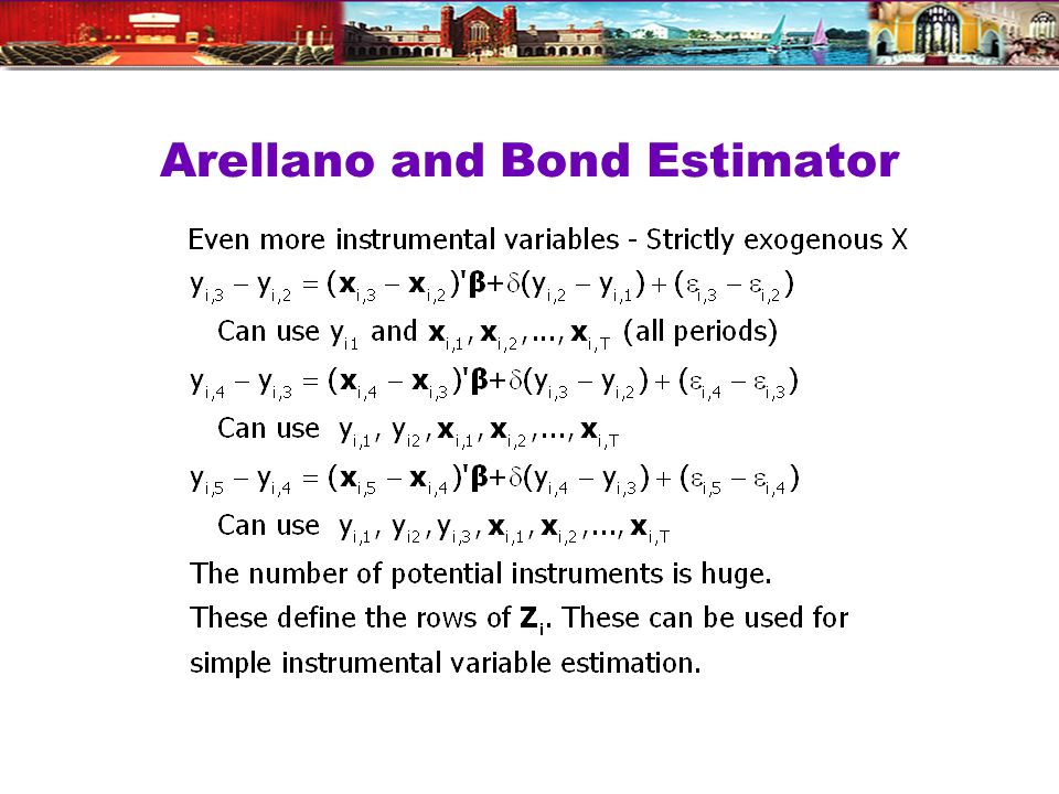
83. Arellano/Bond/Bovers Formulation Builds on Hausman and Taylor

84. Arellano/Bond/Bovers Formulation Adds a Lagged DV to H&T This formulation is the same as H&T with y i,t-1 contained in x2 it.

85. Dynamic (Linear) Panel Data (DPD) Models Application Bias in Conventional Estimation Development of Consistent Estimators Efficient GMM Estimators

86. Dynamic Linear Model

87. A General DPD model

88. Arellano and Bond Estimator

91. Application: Maquiladora http://www.dallasfed.org/news/research/2005/05us-mexico_felix.pdf

92. Maquiladora

93. Estimates