1. The CSISS.org Web Site

2. CSISS.org/Spatial Tools/Toblers Flow Mapper

5. Some nice properties of the program Simple and quick flow map preparation. Extensive color styles available. Black & white too. Hovering over a band or arrow gives the magnitude. Hovering over a centroid gives its label. Two-way, total, or net movement maps. Many to many, one to many, or many to one maps. Easy threshold choice. Some statistics made available. Size dependant only on memory availability. Multiple output formats. Non-geographic flows within firms, industries, organizations, too. Help file included. Microsoft Windows compatible.

6. Flow Mapper Tutorial Parts I, II, III To be used in conjunction with the Flow Mapper program developed by Waldo Tobler & David Jones and available for download at CSISS.org/tools

7. Tutorial Part I General Instructions Getting started The help file also contains instructions

8. The help file has good instructions & hints. After looking at the help files you can view this Welcome screen. To close it click on the smaller (the lower one) of the two xs in the upper right corner. Then go through this tutorial and start using the program.

9. The first steps You will need to have available coordinates and an interaction table. The order in which you load these is not important. I usually load a background map first to make certain that I am working with the correct area, as in the next view. Then I load the locations and place names.

10. Load a background map

11. Locate the file containing the background map Then load it. Or look at it to see the simple format.

12. Boundary Coordinates Number of points, counter-clockwise order, first-last, arbitrary units

13. Background map selected

14. Next: Load locations

15. Select centroid coordinate file Then load it,

16. Locations (centroids) loaded

17. Then: Load location names

18. Select location names file Then load it.

19. Location names selected

20. Load interaction table

21. Select interaction table Then load it

22. Interaction table loaded

23. Select EDIT from the menu

24. Project settings menu selected

25. Flow types: Gross, net, two-way; single row or column or all Sort: Large/small on top, large recommended Line Width: fixed, proportional, maximum size

26. Flow band properties Solid color, gradient, arrowhead style, edge color options

27. Color selection menu Note RGB values. Click OK after choosing.

28. Color appears in flow band box Gradient available in three colors. Edge color helpful when overlaps occur.

29. Threshold None (all flows), average, percent, specific, maximum expected. Note that the average calculated from the interaction table is of all array entries and that the gross flows may exceed this and net flows can be much smaller.

30. Centroid point display None, circle, square, triangle; color, size, edge

31. Background color and title One or two line title moves with FGVT keys when cursor is clicked on map. Back-slash separates title lines

32. To make a map click on the rightmost icon on the second line in the upper left.

33. Here is a map on the screen Ctrl & Alt keys and right mouse can modify it to make it fit. Use right scroll bar too.

34. To save the map Use the little flagged box at the upper left corner; name it with with an extension. All of the map must be on view on the screen! Later cropping may be desirable.

35. To move back to first menu click on flow properties Upper left just below Project Settings

36. For a new map click the Edit option again. This brings up the Project Setting menu. Change the settings as desired for a new map.

37. Settings changed for a net flow map with changed symbol width

38. Arrow style changed simple, standard, barbed

39. Displaying locations with a white circle.

40. Changing map color

41. Changing title

42. Creating new map.

43. New map displayed Save it if it looks good

44. To get moves from (or to) only one place use the Calculate Selected Location Flow on the Flow Type menu

45. Next highlight a row (for from a place) or a column (for to a place) on the interaction table. Or click on the place in the location table. One click gets you the to place, two gets the from place. If you cannot see the interaction table use the view tab in the top line. The map that you get will be of the net flow, so chose an arrowhead style.

46. Or view the interaction table and click on a row

47. The moves from the South Atlantic Division

48. Or moves to the South Atlantic Division Notice choice of arrowhead type

49. The moves to the South Atlantic Division

50. The Flow Mapper program can be downloaded from CSISS.org/Spatial tools. Included are examples and references. Comments and questions can be directed to W. Tobler. http://www.geog.ucsb.edu/~tobler

51. End of part 1 of the tutorial Now experiment with your own data or try some of the files that came with the program in the Data Sets folder, or continue with part 2 of the tutorial.

52. Tutorial Part II An example of using Flow Mapper by Waldo Tobler

53. The life history of a flow mapping project Locate an interaction table. Locate a map. Digitize the map. Enter the table and coordinates. Use the flow map program. Use a model to estimate the movement. Compare the observed with the estimate.

54. Study area in Pennsylvania Ten counties containing five parks

55. Getting coordinates Area outline and centroids, using graph paper.

56. My recording of coordinates

57. Boundary outline coordinates

58. Fifteen centroid coordinates Ten counties and five parks

59. County, then park, names

60. Movement table From 10 counties to 5 parks

61. Having found an interaction matrix, the next step is to get it into the computer If the table is small you can enter it by typing it into notepad. Larger tables can be entered using a spread sheet. Excel tables can be used by converting them to space or comma delimited ASCII files (do not use tab delimited).

62. The 15 by 15 observed movement table. The 10 by 5 table has been forced into a square format. The movement from the 10 counties to the 5 parks is one directional only. The next step is to produce the map, as in the previous tutorial

63. There are visitors from 10 counties to 5 parks The moves indicated are from the counties to the parks. This yields a rectangular table. The flow program expects a square table. The rectangular table needs to be converted to a square table. This is done by constructing a 15 by 15 table, of mostly zeros. The rectangular 10 by 5 table shows up in the upper right hand corner. The full table could show moves between counties & between parks. These moves are not recoded. Return moves are implicit but not depicted. The lower left corner could be used for these, as the transposed table, a 5 by 10 table.

64. Visits by county residents to parks

65. Distance from parks to counties Needed for model estimates. The model also uses the table marginals. These values must also be in a computer file.

66. Movement table From 10 counties to 5 parks with marginals: Insums and Outsums noted

67. Estimated table using the QTP model See QTP.doc under reprints on my web site for a description of the model.

68. Estimated Moves

69. Observed Moves versus QTP Estimated Moves Park attendance

70. Difference: Observed minus Estimated Quadratic transportation model

72. Thank you for your attention Questions can be addressed to: Waldo Tobler Professor Emeritus Geography Department University of California Santa Barbara, CA 93016-4060 http://www.geog.ucsb.edu/~tobler

73. End of part 2 of the tutorial Now experiment with your own data or try some of the files that came with the program in the Data Sets folder, or continue with part 3 of the tutorial

74. Tutorial Part III Examples produced using the Flow Mapper program. by Waldo Tobler

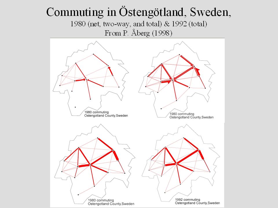
75. Two-way, Total (Gross), and Net Migration

76. Showing 2256 flows from 48 by 48 table, with constant width bands

77. 1995-2000 Total Migration Variable width bands.

78. 1995-2000 Net Migration Complete and simplified.

79. 1995-2000 Migration from and to California Flows from CAMajor flows to CA

80. 1995-2000 Net Migration by two age groups, and movement size.

81. Migration Patterns Persist the Netherlands 1984 1994

82. Net Migration in the United States US Census Data 1985-1990 1995-2000

83. Difference between 1985-1990 and 1995-2000 Migration US Census information

84. Migration by Census Divisions Top: 1965-1970 Migration, Total and Net Bottom: Birth to 1970 Residence, Total and Net

85. Gross and Net Moves M ij + M ji and |M ij - M ji |

86. Variations in style With islands, showing centroids, and title.

87. Legend Box A legend box (an island) with gross moves. Numbers added later.

88. Legend box for net moves

89. London 1965-1966 Inter-borough migration from 33 boroughs. Exploration of map styles, especially colors,

90. Commuting Pattern in Roanoke, VA, 1965 By Census Tract

92. Transfers between eleven schools in Santa Barbara School locations adjusted for clarity. Courtesy of Dr. Stuart Sweeney.

95. Journal to journal referrals between scientific fields

96. End of Tutorial Thank You For Your Attention NOW experiment with your own data or try some of the files that came with the program in the Data Sets folder, or repeat part 1 of the tutorial.

97. Comments or samples of your work done with the flow mapper program are appreciated. Send them to: Waldo Tobler Professor Emeritus Geography department University of California Santa Barbara, CA 93106-4060 http://www.geog.ucsb.edu/~tobler