Download presentation
Presentation is loading. Please wait.

1
3 7 Chapter The Normal Probability Distribution
© 2010 Pearson Prentice Hall. All rights reserved

2
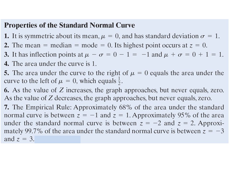
Section 7.1 Properties of the Normal Distribution
© 2010 Pearson Prentice Hall. All rights reserved

4
EXAMPLE Illustrating the Uniform Distribution
Suppose that United Parcel Service is supposed to deliver a package to your front door and the arrival time is somewhere between 10 am and 11 am. Let the random variable X represent the time from10 am when the delivery is supposed to take place. The delivery could be at 10 am (x = 0) or at 11 am (x = 60) with all 1-minute interval of times between x = 0 and x = 60 equally likely. That is to say your package is just as likely to arrive between 10:15 and 10:16 as it is to arrive between 10:40 and 10:41. The random variable X can be any value in the interval from 0 to 60, that is, 0 < X < 60. Because any two intervals of equal length between 0 and 60, inclusive, are equally likely, the random variable X is said to follow a uniform probability distribution.
 or at 11 am (x = 60) with all 1-minute interval of times between x = 0 and x = 60 equally likely. That is to say your package is just as likely to arrive between 10:15 and 10:16 as it is to arrive between 10:40 and 10:41. The random variable X can be any value in the interval from 0 to 60, that is, 0 < X < 60. Because any two intervals of equal length between 0 and 60, inclusive, are equally likely, the random variable X is said to follow a uniform probability distribution.")
6
The graph below illustrates the properties for the “time” example
The graph below illustrates the properties for the “time” example. Notice the area of the rectangle is one and the graph is greater than or equal to zero for all x between 0 and 60, inclusive. Because the area of a rectangle is height times width, and the width of the rectangle is 60, the height must be 1/60.

7
Values of the random variable X less than 0 or greater than 60 are impossible, thus the equation must be zero for X less than 0 or greater than 60.

8
The area under the graph of the density function over an interval represents the probability of observing a value of the random variable in that interval.

9
EXAMPLE Area as a Probability
The probability of choosing a time that is between 15 and 30 seconds after the minute is the area under the uniform density function. Area = P(15 < x < 30) = 15/60 = 0.25
 = 15/60. =")
10
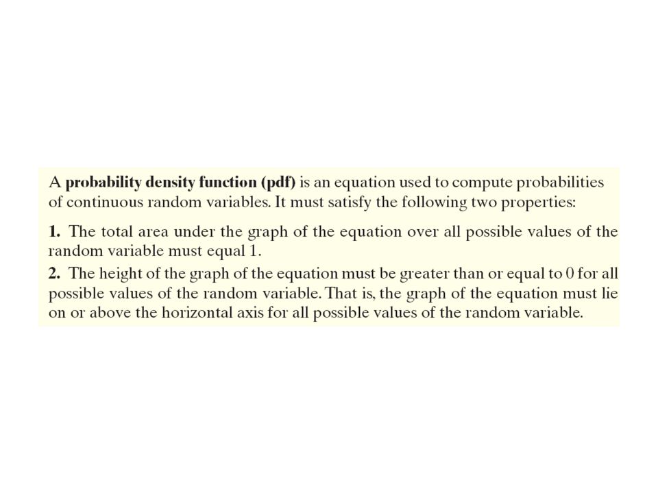
A probability density function
(a) Shows the number of observations for a variable (b) Lists the probabilities for a discrete random variable (c) Shows how dense the mean and standard deviation are compared to the median (d) Is used to compute probabilities for continuous random variables (e) Not sure
 Shows the number of observations for a variable. (b) Lists the probabilities for a discrete random variable. (c) Shows how dense the mean and standard deviation are compared to the median. (d) Is used to compute probabilities for continuous random variables. (e) Not sure.")
11
True or False: The area under a probability density function must equal 1.

13
Relative frequency histograms that are symmetric and bell-shaped are said to have the shape of a normal curve.

14
If a continuous random variable is normally distributed, or has a normal probability distribution, then a relative frequency histogram of the random variable has the shape of a normal curve (bell-shaped and symmetric).
.")
16
The curve below is not a normal curve because
(a) It is skewed left (b) It is not continuous (c) It is skewed right (d) It has outliers (e) Not sure
 It is skewed left. (b) It is not continuous. (c) It is skewed right. (d) It has outliers. (e) Not sure.")
17
What is the mean of the normal distribution shown?
(c) 140 (d) 100 (e) Not sure
 140. (d) 100. (e) Not sure.")
18
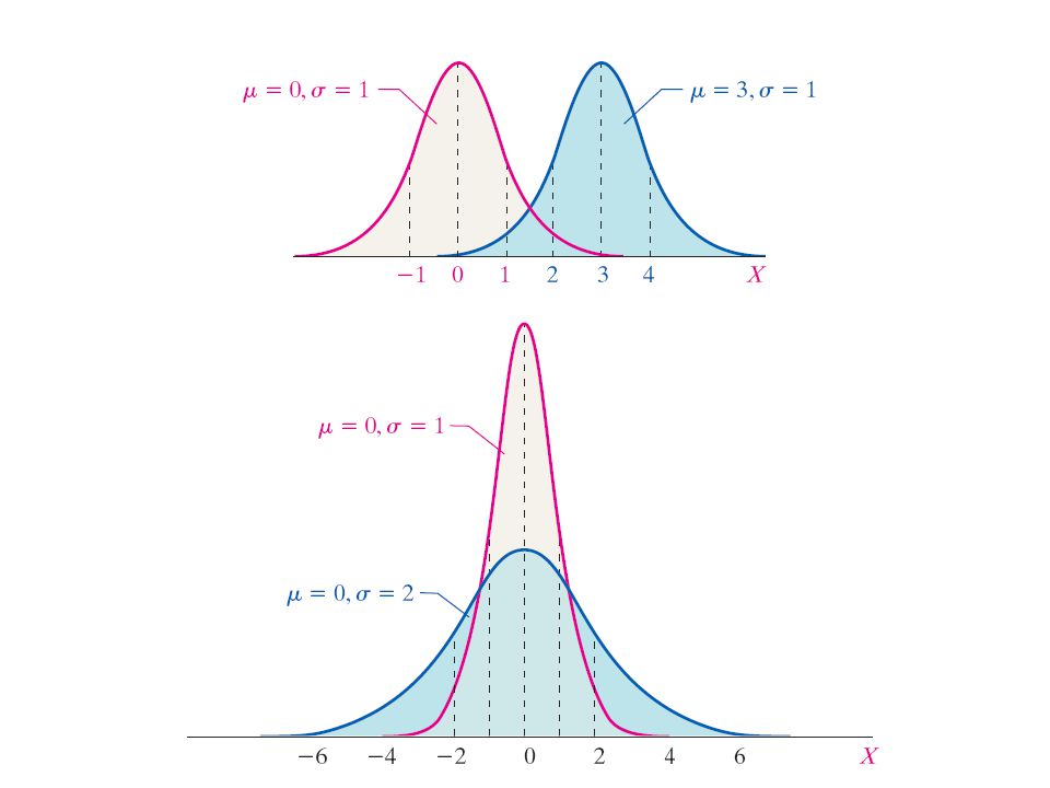
Each graph represents a normal curve with mean μ = 100
Each graph represents a normal curve with mean μ = 100. Which graph indicates the normal random variable X has more dispersion? (a) Blue graph (b) Red graph (c) Not sure
 Blue graph. (b) Red graph. (c) Not sure.")
22
The normal density curve
(a) Is not symmetric (b) Has an area under the curve equal to one. (c) Always has a mean of 0 (d) Has positive and negative values (e) Not sure
 Is not symmetric. (b) Has an area under the curve equal to one. (c) Always has a mean of 0. (d) Has positive and negative values. (e) Not sure.")
24
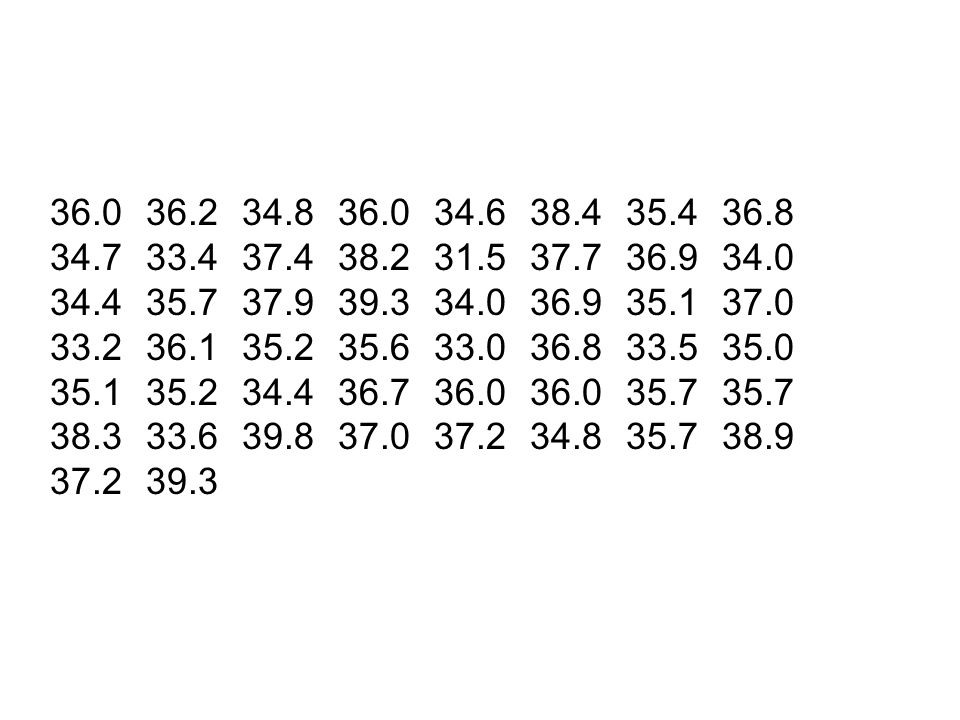
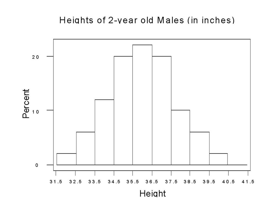
EXAMPLE A Normal Random Variable
The data on the next slide represent the heights (in inches) of a random sample of 50 two-year old males. (a) Draw a histogram of the data using a lower class limit of the first class equal to 31.5 and a class width of 1. (b) Do you think that the variable “height of 2-year old males” is normally distributed?
 of a random sample of 50 two-year old males. (a) Draw a histogram of the data using a lower class limit of the first class equal to 31.5 and a class width of 1. (b) Do you think that the variable height of 2-year old males is normally distributed")
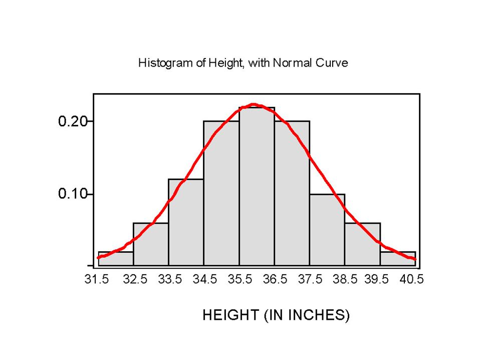
27
In the next slide, we have a normal density curve drawn over the histogram. How does the area of the rectangle corresponding to a height between 34.5 and 35.5 inches relate to the area under the curve between these two heights?

31
EXAMPLE Interpreting the Area Under a Normal Curve
The weights of giraffes are approximately normally distributed with mean μ = 2200 pounds and standard deviation σ = 200 pounds. Draw a normal curve with the parameters labeled. Shade the area under the normal curve to the left of x = 2100 pounds. Suppose that the area under the normal curve to the left of x = 2100 pounds is Provide two interpretations of this result. (a), (b) (c) The proportion of giraffes whose weight is less than 2100 pounds is The probability that a randomly selected giraffe weighs less than 2100 pounds is
, (b) (c) The proportion of giraffes whose weight is less than 2100 pounds is The probability that a randomly selected giraffe weighs less than 2100 pounds is")
34
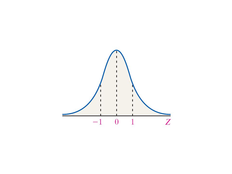
EXAMPLE. Relation Between a Normal Random Variable and a
EXAMPLE Relation Between a Normal Random Variable and a Standard Normal Random Variable The weights of giraffes are approximately normally distributed with mean μ = 2200 pounds and standard deviation σ = 200 pounds. Draw a graph that demonstrates the area under the normal curve between 2000 and 2300 pounds is equal to the area under the standard normal curve between the Z-scores of 2000 and 2300 pounds.

35
Section 7.2 The Standard Normal Distribution

39
The area to the right of 0 under the standard normal curve is equal to
(b) 0.25 (c) 0.5 (d) 1.0 (e) Not sure
 (c) 0.5. (d) 1.0. (e) Not sure.")
40
If the area to the right of 0
If the area to the right of 0.41 under the standard normal curve is equal to 0.34, then the area to the left of 0.41 is equal to (a) 0.66 (b) 0.50 (c) 0.34 (d) 0.17 (e) Not sure
 (b) (c) (d) (e) Not sure.")
42
The table gives the area under the standard normal curve for values to the left of a specified Z-score, zo, as shown in the figure.

43
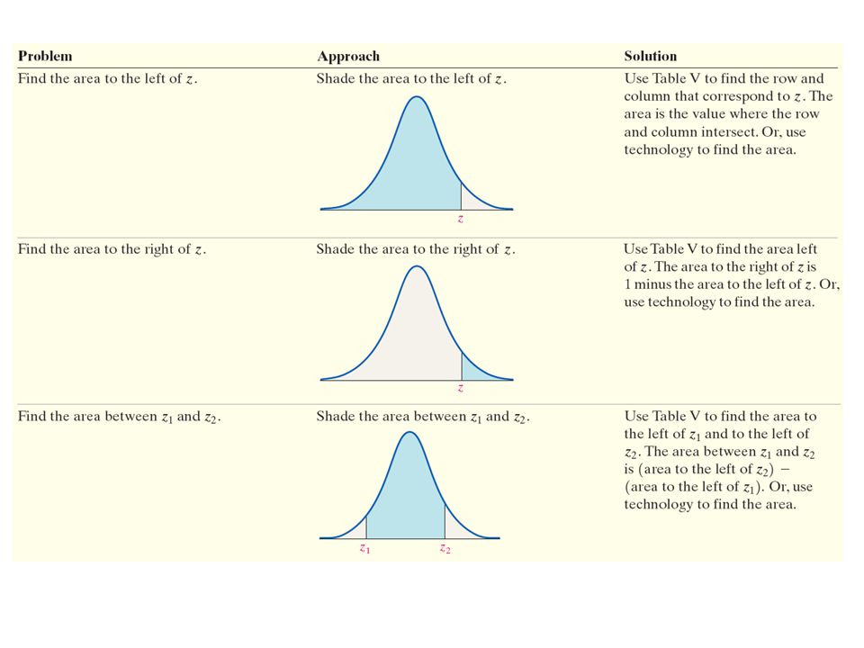
EXAMPLE Finding the Area Under the Standard Normal Curve
Find the area under the standard normal curve to the left of z = Area left of z = is

44
Find the area under the standard normal curve to the left of z = 1.54.

45
Area under the normal curve to the right of zo = 1 – Area to the left of zo

46
EXAMPLE Finding the Area Under the Standard Normal Curve
Find the area under the standard normal curve to the right of Z = 1.25. Area right of 1.25 = 1 – area left of 1.25 = 1 – =

47
Find the area under the standard normal curve to the right of z = -2

48
EXAMPLE Finding the Area Under the Standard Normal Curve
Find the area under the standard normal curve between z = and z = 2.94. Area between and 2.94 = (Area left of z = 2.94) – (area left of z = -1.02) = – =
 – (area left of z = -1.02) = – =")
51
EXAMPLE Finding a z-score from a Specified Area to the Left
Find the z-score such that the area to the left of the z-score is The z-score such that the area to the left of the z-score is is z = 0.57.

52
EXAMPLE Finding a z-score from a Specified Area to the Right
Find the z-score such that the area to the right of the z-score is The area left of the z-score is 1 – = The approximate z-score that corresponds to an area of to the left ( to the right) is Therefore, z = 0.52.
 is Therefore, z =")
53
EXAMPLE Finding a z-score from a Specified Area
Find the z-scores that separate the middle 92% of the area under the normal curve from the 8% in the tails. Area = 0.8 Area = 0.1 Area = 0.1 z1 is the z-score such that the area left is 0.1, so z1 = z2 is the z-score such that the area left is 0.9, so z2 = 1.28.

54
The notation zα (prounounced “z sub alpha”) is the z-score such that the area under the standard normal curve to the right of zα is α.
 is the z-score such that the area under the standard normal curve to the right of zα is α.")
55
EXAMPLE Finding the Value of z
Find the value of z0.25 We are looking for the z-value such that the area to the right of the z-value is This means that the area left of the z-value is 0.75. z0.25 = 0.67

56
The notation zα is The Z-score such that the area under the standard normal curve to the left of zα is α. The Z-score such that the area under the standard normal curve to the right of zα is α. The Z-score such that the area under the standard normal curve between -zα and zα is α. Not sure

57
Find z0.35

59
Notation for the Probability of a Standard Normal Random Variable
P(a < Z < b) represents the probability a standard normal random variable is between a and b P(Z > a) represents the probability a standard normal random variable is greater than a. P(Z < a) represents the probability a standard normal random variable is less than a.
 represents the probability a standard normal random variable is between a and b. P(Z > a) represents the probability a standard normal random variable is greater than a. P(Z < a) represents the probability a standard normal random variable is less than a.")
60
EXAMPLE Finding Probabilities of Standard Normal Random Variables
Find each of the following probabilities: (a) P(Z < -0.23) (b) P(Z > 1.93) (c) P(0.65 < Z < 2.10) (a) P(Z < -0.23) = (b) P(Z > 1.93) = (c) P(0.65 < Z < 2.10) =
 P(Z < -0.23) (b) P(Z > 1.93) (c) P(0.65 < Z < 2.10) (a) P(Z < -0.23) = (b) P(Z > 1.93) = (c) P(0.65 < Z < 2.10) =")
61
For any continuous random variable, the probability of observing a specific value of the random variable is 0. For example, for a standard normal random variable, P(a) = 0 for any value of a. This is because there is no area under the standard normal curve associated with a single value, so the probability must be 0. Therefore, the following probabilities are equivalent: P(a < Z < b) = P(a < Z < b) = P(a < Z < b) = P(a < Z < b)
 = P(a < Z < b) = P(a < Z < b) = P(a < Z < b)")
62
Section 7.3 Applications of the Normal Distribution

65
EXAMPLE Finding the Probability of a Normal Random Variable
It is known that the length of a certain steel rod is normally distributed with a mean of 100 cm and a standard deviation of 0.45 cm.* What is the probability that a randomly selected steel rod has a length less than 99.2 cm? Interpretation: If we randomly selected 100 steel rods, we would expect about 4 of them to be less than 99.2 cm. *Based upon information obtained from Stefan Wilk.

66
EXAMPLE Finding the Probability of a Normal Random Variable
It is known that the length of a certain steel rod is normally distributed with a mean of 100 cm and a standard deviation of 0.45 cm. What is the probability that a randomly selected steel rod has a length between 99.8 and cm? Interpretation: If we randomly selected 100 steel rods, we would expect about 42 of them to be between 99.8 cm and cm.

67
EXAMPLE Finding the Percentile Rank of a Normal Random Variable
The combined (verbal + quantitative reasoning) score on the GRE is normally distributed with mean 1049 and standard deviation 189. (Source: The Department of Psychology at Columbia University in New York requires a minimum combined score of 1200 for admission to their doctoral program. (Source: What is the percentile rank of a student who earns a combined GRE score of 1300? The area under the normal curve is a probability, proportion, or percentile. Here, the area under the normal curve to the left of 1300 represents the percentile rank of the student. Area left of 1300 = Area left of (z = 1.33) = 0.91 (rounded to two decimal places) Interpretation: The student scored at the 91st percentile. This means the student scored better than 91% of the students who took the GRE.
 score on the GRE is normally distributed with mean 1049 and standard deviation 189. (Source: The Department of Psychology at Columbia University in New York requires a minimum combined score of 1200 for admission to their doctoral program. (Source: What is the percentile rank of a student who earns a combined GRE score of 1300 The area under the normal curve is a probability, proportion, or percentile. Here, the area under the normal curve to the left of 1300 represents the percentile rank of the student. Area left of 1300 = Area left of (z = 1.33) = 0.91 (rounded to two decimal places) Interpretation: The student scored at the 91st percentile. This means the student scored better than 91% of the students who took the GRE.")
68
EXAMPLE. Finding the Proportion Corresponding to a Normal
EXAMPLE Finding the Proportion Corresponding to a Normal Random Variable It is known that the length of a certain steel rod is normally distributed with a mean of 100 cm and a standard deviation of 0.45 cm. Suppose the manufacturer must discard all rods less than 99.1 cm or longer than cm. What proportion of rods must be discarded? The proportion is the area under the normal curve to the left of 99.1 cm plus the area under the normal curve to the right of cm. Area left of area right of = (Area left of z = -2) + (Area right of z = 2) = = Interpretation: The proportion of rods that must be discarded is If the company manufactured 1000 rods, they would expect to discard about 46 of them.
 + (Area right of z = 2) = = Interpretation: The proportion of rods that must be discarded is If the company manufactured 1000 rods, they would expect to discard about 46 of them.")
69
If X is a normal random variable with a mean equal to 4 and a standard deviation equal to 2, then find P(X > 3). Round your answer to four decimal places.

72
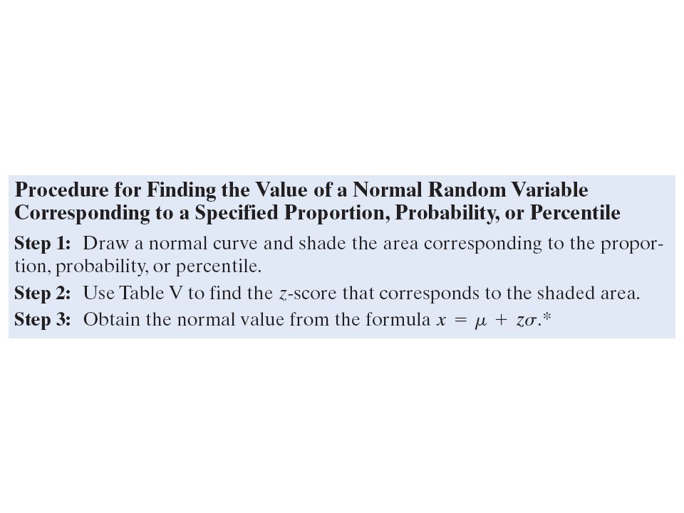
EXAMPLE Finding the Value of a Normal Random Variable
The combined (verbal + quantitative reasoning) score on the GRE is normally distributed with mean 1049 and standard deviation 189. (Source: What is the score of a student whose percentile rank is at the 85th percentile? The z-score that corresponds to the 85th percentile is the z-score such that the area under the standard normal curve to the left is This z-score is 1.04. x = µ + zσ = (189) = 1246 Interpretation: The proportion of rods that must be discarded is If the company manufactured 1000 rods, they would expect to discard about 46 of them.
 score on the GRE is normally distributed with mean 1049 and standard deviation 189. (Source: What is the score of a student whose percentile rank is at the 85th percentile The z-score that corresponds to the 85th percentile is the z-score such that the area under the standard normal curve to the left is This z-score is x = µ + zσ. = (189) = Interpretation: The proportion of rods that must be discarded is If the company manufactured 1000 rods, they would expect to discard about 46 of them.")
74
IQ scores are normally distributed with mean 100 and standard deviation 15. What IQ score is at the 45th percentile? Round your answer to the nearest whole number.

75
EXAMPLE Finding the Value of a Normal Random Variable
It is known that the length of a certain steel rod is normally distributed with a mean of 100 cm and a standard deviation of 0.45 cm. Suppose the manufacturer wants to accept 90% of all rods manufactured. Determine the length of rods that make up the middle 90% of all steel rods manufactured. z1 = and z2 = 1.645 Area = 0.05 Area = 0.05 x1 = µ + z1σ = (-1.645)(0.45) = cm x2 = µ + z2σ = (1.645)(0.45) = cm Interpretation: The length of steel rods that make up the middle 90% of all steel rods manufactured would have lengths between cm and cm.
(0.45) = cm. x2 = µ + z2σ. = (1.645)(0.45) = cm. Interpretation: The length of steel rods that make up the middle 90% of all steel rods manufactured would have lengths between cm and cm.")
76
Section 7.4 Assessing Normality

77
Suppose that we obtain a simple random sample from a population whose distribution is unknown. Many of the statistical tests that we perform on small data sets (sample size less than 30) require that the population from which the sample is drawn be normally distributed. Up to this point, we have said that a random variable X is normally distributed, or at least approximately normal, provided the histogram of the data is symmetric and bell-shaped. This method works well for large data sets, but the shape of a histogram drawn from a small sample of observations does not always accurately represent the shape of the population. For this reason, we need additional methods for assessing the normality of a random variable X when we are looking at sample data.
 require that the population from which the sample is drawn be normally distributed. Up to this point, we have said that a random variable X is normally distributed, or at least approximately normal, provided the histogram of the data is symmetric and bell-shaped. This method works well for large data sets, but the shape of a histogram drawn from a small sample of observations does not always accurately represent the shape of the population. For this reason, we need additional methods for assessing the normality of a random variable X when we are looking at sample data..")
79
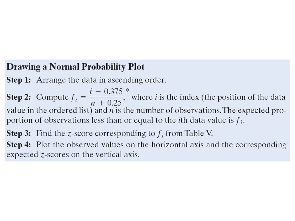
A normal probability plot plots observed data versus normal scores.
A normal score is the expected Z-score of the data value if the distribution of the random variable is normal. The expected Z-score of an observed value will depend upon the number of observations in the data set.

81
The idea behind finding the expected Z-score is that if the data comes from a population that is normally distributed, we should be able to predict the area left of each of the data values. The value of fi represents the expected area left of the ith data value assuming the data comes from a population that is normally distributed. For example, f1 is the expected area left of the smallest data value, f2 is the expected area left of the second smallest data value, and so on.

82
If sample data is taken from a population that is normally distributed, a normal probability plot of the actual values versus the expected Z-scores will be approximately linear.

83
We will be content in reading normal probability plots constructed using the statistical software package, MINITAB. In MINITAB, if the points plotted lie within the bounds provided in the graph, then we have reason to believe that the sample data comes from a population that is normally distributed.

84
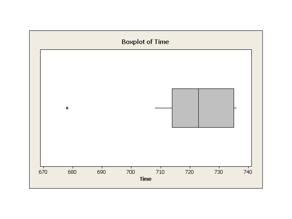
EXAMPLE Interpreting a Normal Probability Plot
The following data represent the time between eruptions (in seconds) for a random sample of 15 eruptions at the Old Faithful Geyser in California. Is there reason to believe the time between eruptions is normally distributed?
 for a random sample of 15 eruptions at the Old Faithful Geyser in California. Is there reason to believe the time between eruptions is normally distributed")
85
The random variable “time between eruptions” is likely not normal.

87
EXAMPLE Interpreting a Normal Probability Plot
Suppose that seventeen randomly selected workers at a detergent factory were tested for exposure to a Bacillus subtillis enzyme by measuring the ratio of forced expiratory volume (FEV) to vital capacity (VC). NOTE: FEV is the maximum volume of air a person can exhale in one second; VC is the maximum volume of air that a person can exhale after taking a deep breath. Is it reasonable to conclude that the FEV to VC (FEV/VC) ratio is normally distributed? Shore, N.S.; Greene R.; and Kazemi, H. “Lung Dysfunction in Workers Exposed to Bacillus subtillis Enzyme,” Environmental Research, 4 (1971), pp
 to vital capacity (VC). NOTE: FEV is the maximum volume of air a person can exhale in one second; VC is the maximum volume of air that a person can exhale after taking a deep breath. Is it reasonable to conclude that the FEV to VC (FEV/VC) ratio is normally distributed Shore, N.S.; Greene R.; and Kazemi, H. Lung Dysfunction in Workers Exposed to Bacillus subtillis Enzyme, Environmental Research, 4 (1971), pp")
88
Reasonable to believe that FEV/VC is normally distributed.

Similar presentations


>")


>")
