1. Quantitative Analysis (Statistics Week 8)
FDA B&M Level C Peter Matthews

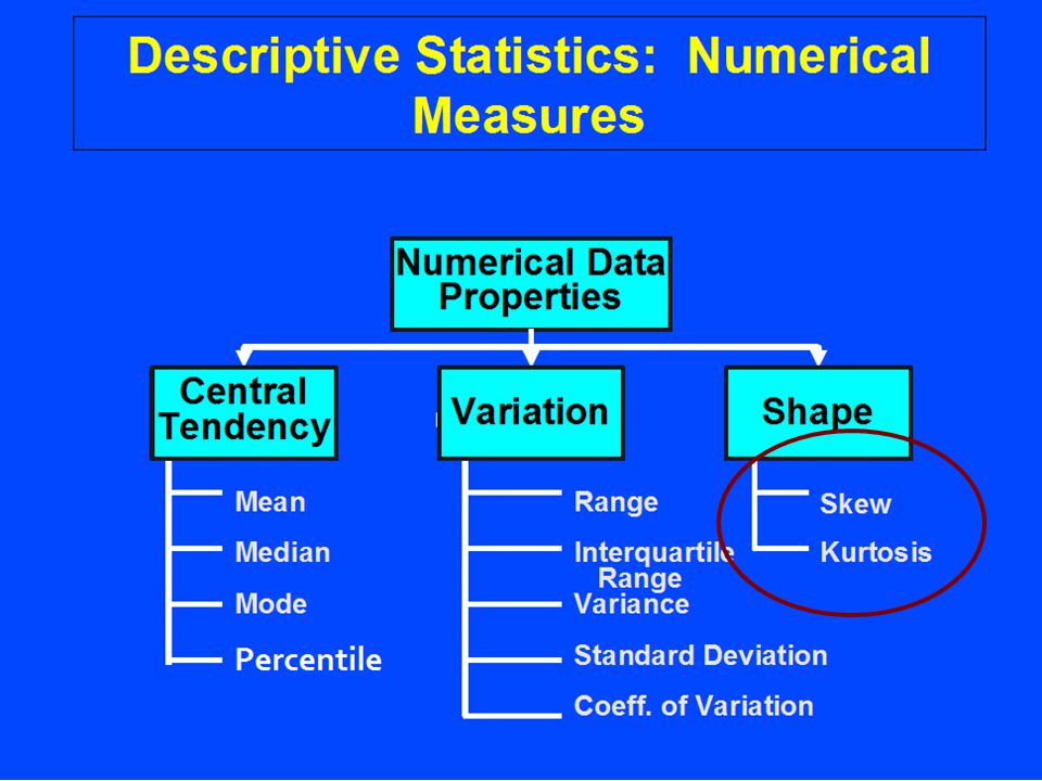
3. Calculating Standard Deviation
1. Find the mean average of the set
2. For each number, subtract
the average from it.
3. Square each of the differences.
4. Add up all the results from Step 3.
5. Divide the sum of squares (Step 4)
by the count of numbers in the data set
, minus one (n–1).
6. Take the Square Root now gives
standard deviation.

4. What is the standard deviation (in English)
By far the most commonly used measure of variability is the standard deviation. The standard deviation of a data set, denoted by s, represents the typical distance from any point in the data set to the centre It’s roughly the average distance from the centre, and in this case, the centre is the average. Most often, you don’t hear a standard deviation given just by itself; if it’s reported (and it’s not reported nearly enough) it’s usually in the fine print, in parentheses, like “(s = 2.68).”

5. Standard Deviation symbol
σ (Population)
S (sample)
Stdev (if in doubt)

6. Here are some properties that can help you when interpreting a standard deviation:
✓ The standard deviation can never be a negative number.
✓ The smallest possible value for the standard deviation is 0 (when every number in the data set is exactly the same).
✓ Standard deviation is affected by outliers, as it’s based on distance from the mean, which is affected by outliers.
✓ The standard deviation has the same units as the original data, while variance is in square units.

8. As we continued to plot foot lengths, a pattern would begin to emerge.
Suppose we measured the right foot length of 30 Students and graphed the results.
Assume the first person had a Size 10 foot. We could create a bar graph and plot that person on the graph.
If our second subject had a size 9 foot, we would add them to the graph.
As we continued to plot foot lengths, a pattern would begin to emerge. 8 7 6 5 4 3 2 1
Number of People with
that Shoe Size
Size of Right Foot

9. Notice how there are more people (n=6) with a size 10 right foot than any other length. Notice also how as the length becomes larger or smaller, there are fewer and fewer people with that measurement. This is a characteristics of many variables that we measure. There is a tendency to have most measurements in the middle, and fewer as we approach the high and low extremes.
If we were to connect the top of each bar, we would create a frequency polygon. 8 7 6 5 4 3 2 1
Number of People with
that Shoe Size
Size of Right Foot

10. You will notice that if we smooth the lines, our data almost creates a bell shaped curve.8 7 6 5 4 3 2 1
Number of People with
that Shoe Size
Size of Right Foot

11. You will notice that if we smooth the lines, our data almost creates a bell shaped curve.
This bell shaped curve is known as the “Bell Curve” or the “Normal Distribution Curve.” 8 7 6 5 4 3 2 1
Number of People with
that Shoe Size
Length of Right Foot

12. Tip of the day :
Whenever you see a normal curve, you should imagine the bar graph within it.
Points on a Quiz
Number of Students 9 8 7 6 5 4 3 2 1

13. Now lets look at quiz scores for 51 students.
Points on a Quiz
Number of Students 9 8 7 6 5 4 3 2 1

14. Mean=17,
= 867
867 / 51 = 17
Points on a Quiz
Number of Students 9 8 7 6 5 4 3 2 1

15. Mean=17,
Mode=17, 12
13 13
21 21 22
Points on a Quiz
Number of Students 9 8 7 6 5 4 3 2 1

16. Median=17,
Mean=17,
Mode=17,
12, 13, 13, 14, 14, 14, 14, 15, 15, 15, 15, 15, 15, 16, 16, 16, 16, 16, 16, 16, 16, 17, 17, 17, 17,
17,
17, 17, 17, 17, 18, 18, 18, 18, 18, 18, 18, 18, 19, 19, 19, 19, 19, 19, 20, 20, 20, 20, 21, 21, 22
Points on a Quiz
Number of Students 9 8 7 6 5 4 3 2 1

17. Will all fall on the same spot for normal distribution
Median=17,
Mean=17,
Mode=17,
Will all fall on the same spot for normal distribution
Points on a Quiz
Number of Students 9 8 7 6 5 4 3 2 1

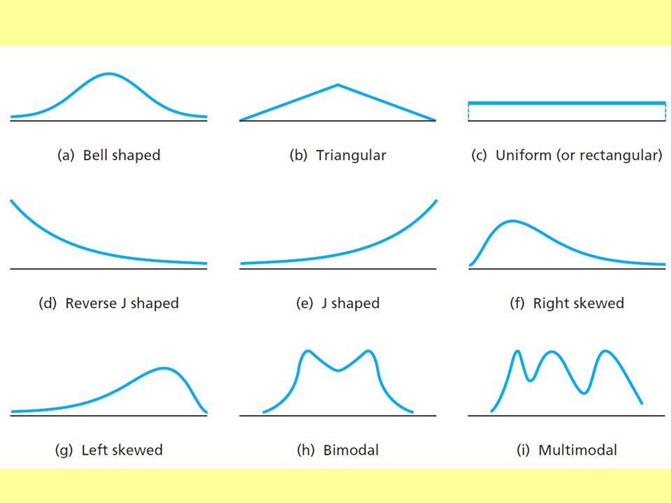
18. Normal distributions (bell shaped) are a family of distributions that have the same general shape. They are symmetric (the left side is an exact mirror of the right side) with scores more concentrated in the middle than in the tails. Examples of normal distributions are shown below. Notice that they differ in how spread out they are. The area under each curve is the same.

19. The Normal Distribution
f(X)
Changing σ/s (stdev) increases or decreases the spread. σ
Mean
Median
Mode X

20. Lower Stdev (narrower)
Higher Stdev (wider)

21. +/- 1 standard deviation
Empirical Rule
For data having a bell-shaped distribution:
of the values of a normal random variable
are within of its mean.
68.26%
+/- 1 standard deviation
of the values of a normal random variable
are within of its mean.
95.44%
+/- 2 standard deviations
of the values of a normal random variable
are within of its mean.
99.72%
+/- 3 standard deviations

22. If your data fits a normal distribution, approximately 68% of your subjects will fall within one standard deviation of the mean.
Approximately 95% of your subjects will fall within two standard deviations of the mean.
Over 99% of your subjects will fall within three standard deviations of the mean.

23. Points on a Different Test
The number of points that one standard deviations equals varies from distribution to distribution. On one maths test, a standard deviation = 7 points. The mean = 45, then we would know that 68% of the students scored from 38 to 52.
Points on Math Test
Points on a Different Test
On another test, Standard deviation = 5 points. The mean is still 45, then 68% of the students would score from 40 to 50 points.

24. The mean and standard deviation are useful ways to describe a set of scores. If the scores are grouped closely together, they will have a smaller standard deviation than if they are spread farther apart.
Small Standard Deviation
Large Standard Deviation
Comparing Data
Different Means
Different Standard Deviations
Same Standard Deviations
Same Means

25. Skew refers to the tail of the distribution.
Data do not always form a normal distribution. When most of the scores are high, the distributions is not normal, but negatively (left) skewed.
Skew refers to the tail of the distribution.
Because the tail is on the negative (left) side of the graph, the distribution has a negative (left) skew. 8 7 6 5 4 3 2 1
Number of People with
that Shoe Size
Size of Right Foot

26. When most of the scores are low, the distributions is not normal, but positively (right) skewed.
Because the tail is on the positive (right) side of the graph, the distribution has a positive (right) skew. 8 7 6 5 4 3 2 1
Number of People with
that Shoe Size
Size of Right Foot

27. When data are skewed, they do not possess the characteristics of the normal curve (distribution). For example, 68% of the subjects do not fall within one standard deviation above or below the mean. The mean, mode, and median do not fall on the same score. The mode will still be represented by the highest point of the distribution, but the mean will be toward the side with the tail and the median will fall between the mode and mean.

30. Class test
33,17,19,25,28,56,12,45,95,52,65,55,62,42,53,61,19,18,25
Calculate Mean, Median, Mode are these numbers a :
Or Something different

31. Questions ?
Next week – scattergraphs, trends, correleation in others words Question 2