Download presentation
Presentation is loading. Please wait.

1
Introduction to SPSS 16.0 1

2
Review of Concepts (stats and scales) Data entry (the workspace and labels) – By hand – Import Excel Running an analysis- frequency, central tendency, correlation 2
 Data entry (the workspace and labels) – By hand – Import Excel Running an analysis- frequency, central tendency, correlation 2")
3
Types of Statistics Descriptive- summarize or describe our observations Inferential- use observations to allow us to make predictions (inferences) about a situation that has not yet occurred 3
 about a situation that has not yet occurred 3")
4
Descriptive or Inferential? a)I cycle about 50 km per week on average. b)We can expect a lot of rain this time of year. 4 Rowntree, D. (1981). Statistics without tears. London: Penguin Books.
We can expect a lot of rain this time of year. 4 Rowntree, D. (1981). Statistics without tears. London: Penguin Books..")
5
Population vs Sample A population refers to all the cases to which a researcher wants his estimates to apply to – White mice, lightbulb life, students A sample is used because it is normally impossible to study all the members of a population Descriptive stats simply summarize a sample Inferential stats generalize from a sample to the wider population 5

6
Variables Samples are made up of individuals, all individuals have characteristics. Members of a sample will differ on certain characteristics. Hence, we call this variation amongst individuals variable characteristics or variables for short. 6 Rowntree, D. (1981). Statistics without tears. London: Penguin Books.
. Statistics without tears. London: Penguin Books..")
7
Types of Variables What are variables you would consider in buying a second hand bike? Brand (Trek, Raleigh) Type (road, mountain, racer) Components (Shimano, no name) Age Condition (Excellent, good, poor) Price Frame size Number of gears 7 Rowntree, D. (1981). Statistics without tears. London: Penguin Books.
 Type (road, mountain, racer) Components (Shimano, no name) Age Condition (Excellent, good, poor) Price Frame size Number of gears 7 Rowntree, D. (1981). Statistics without tears. London: Penguin Books..")
8
Types of Scales Nominal- objects or people are categorized according to some criterion (gender, job category) Ordinal- Categories which are ranked according to characteristics (income- low, moderate, high) Interval- contain equal distance between units of measure- but no zero (calendar years, temperature) Ratio- has an absolute zero and consistent intervals (distance, weight) 8
 Ordinal- Categories which are ranked according to characteristics (income- low, moderate, high) Interval- contain equal distance between units of measure- but no zero (calendar years, temperature) Ratio- has an absolute zero and consistent intervals (distance, weight) 8")
9
Parametric vs Non-parametric Parametric stats are more powerful than non- parametric stats- for real numbers- T test Non-parametric stats are not as powerful but good for category variables - Mann-Whitney U (likert) 9
 9")
10
The Four Windows: Data editor Output viewer Syntax editor Script window

11
The Four Windows: Data Editor Data Editor Spreadsheet-like system for defining, entering, editing, and displaying data. Extension of the saved file will be “sav.”

12
The Four Windows: Output Viewer Output Viewer Displays output and errors. Extension of the saved file will be “spv.”

13
The Four Windows: Syntax editor Syntax Editor Text editor for syntax composition. Extension of the saved file will be “sps.”

14
The Four Windows: Script Window Script Window Provides the opportunity to write full-blown programs, in a BASIC-like language. Text editor for syntax composition. Extension of the saved file will be “sbs.”

15
The basics of managing data files

16
Opening SPSS Start → All Programs → SPSS Inc→ SPSS 16.0 → SPSS 16.0

17
Opening SPSS The default window will have the data editor There are two sheets in the window: 1. Data view2. Variable view

18
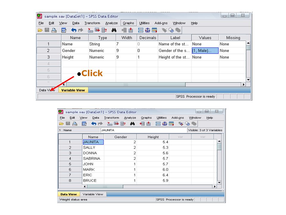
Data View window The Data View window This sheet is visible when you first open the Data Editor and this sheet contains the data Click on the tab labeled Variable View Click

19
Variable View window This sheet contains information about the data set that is stored with the dataset Name –The first character of the variable name must be alphabetic –Variable names must be unique, and have to be less than 64 characters. –Spaces are NOT allowed.

20
Variable View window: Type Type –Click on the ‘type’ box. The two basic types of variables that you will use are numeric and string. This column enables you to specify the type of variable.

21
Variable View window: Width Width –Width allows you to determine the number of characters SPSS will allow to be entered for the variable

22
Variable View window: Decimals Decimals –Number of decimals –It has to be less than or equal to 16

23
Variable View window: Label Label –You can specify the details of the variable –You can write characters with spaces up to 256 characters

24
Variable View window: Values Values –This is used and to suggest which numbers represent which categories when the variable represents a category

25
Defining the value labels Click the cell in the values column as shown below For the value, and the label, you can put up to 60 characters. After defining the values click add and then click OK. Clic k

26
Practice 1 How would you put the following information into SPSS? Value = 1 represents Male and Value = 2 represents Female

27
Practice 1 (Solution Sample) Clic k
 Clic k")
29
Saving the data To save the data file you created simply click ‘file’ and click ‘save as.’ You can save the file in different forms by clicking “Save as type.” Click

30
Sorting the data Click ‘Data’ and then click Sort Cases

31
Sorting the data (cont’d) Double Click ‘Name of the students.’ Then click ok. Cli ck
 Double Click ‘Name of the students.’ Then click ok. Cli ck")
32
Practice 2 How would you sort the data by the ‘Height’ of students in descending order? Answer –Click data, sort cases, double click ‘height of students,’ click ‘descending,’ and finally click ok.

33
Transforming data Click ‘Transform’ and then click ‘Compute Variable…’

34
Transforming data (cont’d) Example: Adding a new variable named ‘lnheight’ which is the natural log of height –Type in lnheight in the ‘Target Variable’ box. Then type in ‘ln(height)’ in the ‘Numeric Expression’ box. Click OK Click
’ in the ‘Numeric Expression’ box. Click OK Click.")
35
Transforming data (cont’d) A new variable ‘lnheight’ is added to the table
 A new variable ‘lnheight’ is added to the table")
36
Practice 3 Create a new variable named “sqrtheight” which is the square root of height. Answer

37
The basic analysis

38
The basic analysis of SPSS that will be introduced in this class Frequencies –This analysis produces frequency tables showing frequency counts and percentages of the values of individual variables. Descriptives –This analysis shows the maximum, minimum, mean, and standard deviation of the variables Linear regression analysis –Linear Regression estimates the coefficients of the linear equation

39
Opening the sample data Open ‘Employee data.sav’ from the SPSS –Go to “File,” “Open,” and Click Data

40
Opening the sample data Go to Program Files,” “SPSSInc,” “SPSS16,” and “Samples” folder. Open “Employee Data.sav” file

41
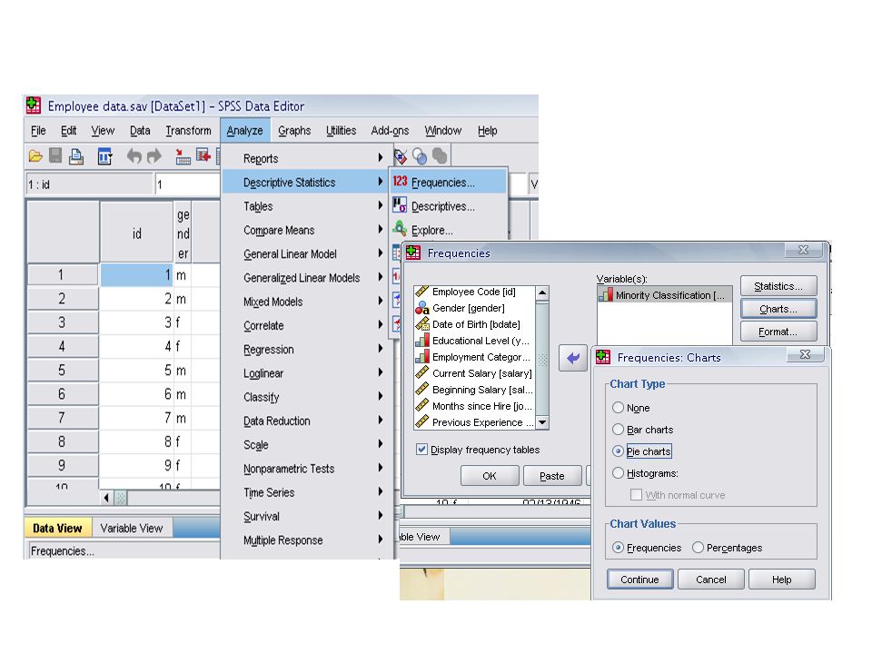
Frequencies Click ‘Analyze,’ ‘Descriptive statistics,’ then click ‘Frequencies’

42
Frequencies Click gender and put it into the variable box. Click ‘Charts.’ Then click ‘Bar charts’ and click ‘Continue.’ Clic k

43
Frequencies Finally Click OK in the Frequencies box. Click

45
Using the Syntax editor Click ‘Analyze,’ ‘Descriptive statistics,’ then click ‘Frequencies.’ Put ‘Gender’ in the Variable(s) box. Then click ‘Charts,’ ‘Bar charts,’ and click ‘Continue.’ Click ‘Paste.’ Click

46
Using the Syntax editor Highlight the commands in the Syntax editor and then click the run icon. You can do the same thing by right clicking the highlighted area and then by clicking ‘Run Current’ Cli ck Righ t Click!

47
Practice 4 Do a frequency analysis on the variable “minority” Create pie charts for it Do the same analysis using the syntax editor

49
Answer Click

50
Descriptives Click ‘Analyze,’ ‘Descriptive statistics,’ then click ‘Descriptives…’ Click ‘Educational level’ and ‘Beginning Salary,’ and put it into the variable box. Click Options Cli ck

51
Descriptives The options allows you to analyze other descriptive statistics besides the mean and Std. Click ‘variance’ and ‘kurtosis’ Finally click ‘Continue’ Click

52
Descriptives Finally Click OK in the Descriptives box. You will be able to see the result of the analysis.

53
Regression Analysis Click ‘Analyze,’ ‘Regression,’ then click ‘Linear’ from the main menu.

54
Regression Analysis For example let’s analyze the model Put ‘Beginning Salary’ as Dependent and ‘Educational Level’ as Independent. Cli ck

55
Regression Analysis Clicking OK gives the result

56
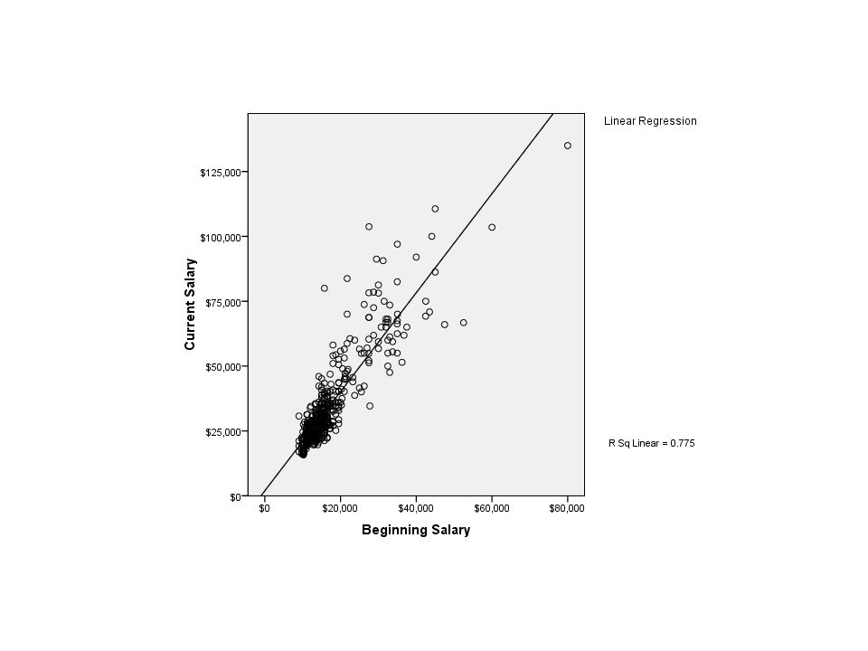
Plotting the regression line Click ‘Graphs,’ ‘Legacy Dialogs,’ ‘Interactive,’ and ‘Scatterplot’ from the main menu.

57
Plotting the regression line Drag ‘Current Salary’ into the vertical axis box and ‘Beginning Salary’ in the horizontal axis box. Click ‘Fit’ bar. Make sure the Method is regression in the Fit box. Then click ‘OK’. Cli ck Set this to Regressi on!

59
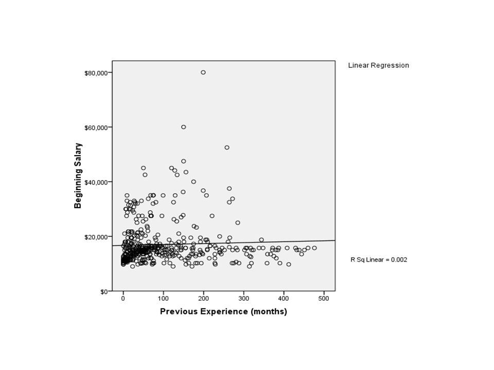
Practice 5 Find out whether or not the previous experience of workers has any affect on their beginning salary? –Take the variable “salbegin,” and “prevexp” as dependent and independent variables respectively. Plot the regression line for the above analysis using the “scatter plot” menu.

60
Answer Cli ck

62
Click on the “fit” tab to make sure the method is regression

Similar presentations


 Data entry (the workspace and labels) –By hand –Import Excel.>")
 (pp.48-58) Chapter 1 Introduction.>")

>")

 Commonly used statistical software.>")

 Kentaka Aruga.>")
 18.0 WINDOWS.>")
>")


151 231 2284 CMPDLLM002 Research Methods Lecture 9: Quantitative.>")


 UNIVERSITY OF WASHINGTON September 17, 2009 Introduction to SPSS (Version 16)>")