Download presentation
Presentation is loading. Please wait.

1
AMwww.Remote-Sensing.info Review Ch.1-6 www.Remote-Sensing.info

2
Ch.1 Remote Sensing and Digital Image Processing www.Remote-Sensing.info

3
ASPRS adopted a combined formal definition of photogrammetry and remote sensing as (Colwell, 1997): “the art, science, and technology of obtaining reliable information about physical objects and the environment, through the process of recording, measuring and interpreting imagery and digital representations of energy patterns derived from noncontact sensor systems”. ASPRS adopted a combined formal definition of photogrammetry and remote sensing as (Colwell, 1997): “the art, science, and technology of obtaining reliable information about physical objects and the environment, through the process of recording, measuring and interpreting imagery and digital representations of energy patterns derived from noncontact sensor systems”. Remote Sensing Data Collection www.Remote-Sensing.info
: the art, science, and technology of obtaining reliable information about physical objects and the environment, through the process of recording, measuring and interpreting imagery and digital representations of energy patterns derived from noncontact sensor systems . Remote Sensing Data Collection")
4
A remote sensing instrument collects information about an object or phenomenon within the instantaneous-field-of-view (IFOV) of the sensor system without being in direct physical contact with it. The sensor is located on a suborbital or satellite platform. A remote sensing instrument collects information about an object or phenomenon within the instantaneous-field-of-view (IFOV) of the sensor system without being in direct physical contact with it. The sensor is located on a suborbital or satellite platform. www.Remote-Sensing.info
 of the sensor system without being in direct physical contact with it. The sensor is located on a suborbital or satellite platform.")
5
Remote sensing is unobtrusive if the sensor passively records the EMR reflected or emitted by the object of interest. Passive remote sensing does not disturb the object or area of interest. Remote sensing is unobtrusive if the sensor passively records the EMR reflected or emitted by the object of interest. Passive remote sensing does not disturb the object or area of interest. Remote sensing devices may be programmed to collect data systematically, such as within a 9 9 in. frame of vertical aerial photography. This systematic data collection can remove the sampling bias introduced in some in situ investigations. Remote sensing devices may be programmed to collect data systematically, such as within a 9 9 in. frame of vertical aerial photography. This systematic data collection can remove the sampling bias introduced in some in situ investigations. Under controlled conditions, remote sensing can provide fundamental biophysical information, including x,y location, z elevation or depth, biomass, temperature, and moisture content. Under controlled conditions, remote sensing can provide fundamental biophysical information, including x,y location, z elevation or depth, biomass, temperature, and moisture content. Remote sensing is unobtrusive if the sensor passively records the EMR reflected or emitted by the object of interest. Passive remote sensing does not disturb the object or area of interest. Remote sensing is unobtrusive if the sensor passively records the EMR reflected or emitted by the object of interest. Passive remote sensing does not disturb the object or area of interest. Remote sensing devices may be programmed to collect data systematically, such as within a 9 9 in. frame of vertical aerial photography. This systematic data collection can remove the sampling bias introduced in some in situ investigations. Remote sensing devices may be programmed to collect data systematically, such as within a 9 9 in. frame of vertical aerial photography. This systematic data collection can remove the sampling bias introduced in some in situ investigations. Under controlled conditions, remote sensing can provide fundamental biophysical information, including x,y location, z elevation or depth, biomass, temperature, and moisture content. Under controlled conditions, remote sensing can provide fundamental biophysical information, including x,y location, z elevation or depth, biomass, temperature, and moisture content. Advantages of Remote Sensing www.Remote-Sensing.info

6
The greatest limitation is that it is often oversold. Remote sensing is not a panacea that provides all the information needed to conduct physical, biological, or social science research. It provides some spatial, spectral, and temporal information of value in a manner that we hope is efficient and economical. The greatest limitation is that it is often oversold. Remote sensing is not a panacea that provides all the information needed to conduct physical, biological, or social science research. It provides some spatial, spectral, and temporal information of value in a manner that we hope is efficient and economical. Human beings select the appropriate remote sensing system to collect the data, specify the various resolutions of the remote sensor data, calibrate the sensor, select the platform that will carry the sensor, determine when the data will be collected, and specify how the data are processed. Human beings select the appropriate remote sensing system to collect the data, specify the various resolutions of the remote sensor data, calibrate the sensor, select the platform that will carry the sensor, determine when the data will be collected, and specify how the data are processed. The greatest limitation is that it is often oversold. Remote sensing is not a panacea that provides all the information needed to conduct physical, biological, or social science research. It provides some spatial, spectral, and temporal information of value in a manner that we hope is efficient and economical. The greatest limitation is that it is often oversold. Remote sensing is not a panacea that provides all the information needed to conduct physical, biological, or social science research. It provides some spatial, spectral, and temporal information of value in a manner that we hope is efficient and economical. Human beings select the appropriate remote sensing system to collect the data, specify the various resolutions of the remote sensor data, calibrate the sensor, select the platform that will carry the sensor, determine when the data will be collected, and specify how the data are processed. Human beings select the appropriate remote sensing system to collect the data, specify the various resolutions of the remote sensor data, calibrate the sensor, select the platform that will carry the sensor, determine when the data will be collected, and specify how the data are processed. Limitations of Remote Sensing www.Remote-Sensing.info

7
Powerful active remote sensor systems that emit their own electromagnetic radiation (e.g., LIDAR, RADAR, SONAR) can be intrusive and affect the phenomenon being investigated. Additional research is required to determine how intrusive these active sensors can be. Powerful active remote sensor systems that emit their own electromagnetic radiation (e.g., LIDAR, RADAR, SONAR) can be intrusive and affect the phenomenon being investigated. Additional research is required to determine how intrusive these active sensors can be. Remote sensing instruments may become uncalibrated, resulting in uncalibrated remote sensor data. Remote sensing instruments may become uncalibrated, resulting in uncalibrated remote sensor data. Remote sensor data may be expensive to collect and analyze. Hopefully, the information extracted from the remote sensor data justifies the expense. Remote sensor data may be expensive to collect and analyze. Hopefully, the information extracted from the remote sensor data justifies the expense. Powerful active remote sensor systems that emit their own electromagnetic radiation (e.g., LIDAR, RADAR, SONAR) can be intrusive and affect the phenomenon being investigated. Additional research is required to determine how intrusive these active sensors can be. Powerful active remote sensor systems that emit their own electromagnetic radiation (e.g., LIDAR, RADAR, SONAR) can be intrusive and affect the phenomenon being investigated. Additional research is required to determine how intrusive these active sensors can be. Remote sensing instruments may become uncalibrated, resulting in uncalibrated remote sensor data. Remote sensing instruments may become uncalibrated, resulting in uncalibrated remote sensor data. Remote sensor data may be expensive to collect and analyze. Hopefully, the information extracted from the remote sensor data justifies the expense. Remote sensor data may be expensive to collect and analyze. Hopefully, the information extracted from the remote sensor data justifies the expense. Limitations of Remote Sensing www.Remote-Sensing.info
 can be intrusive and affect the phenomenon being investigated. Additional research is required to determine how intrusive these active sensors can be. Remote sensing instruments may become uncalibrated, resulting in uncalibrated remote sensor data. Remote sensing instruments may become uncalibrated, resulting in uncalibrated remote sensor data. Remote sensor data may be expensive to collect and analyze. Hopefully, the information extracted from the remote sensor data justifies the expense. Remote sensor data may be expensive to collect and analyze. Hopefully, the information extracted from the remote sensor data justifies the expense. Powerful active remote sensor systems that emit their own electromagnetic radiation (e.g., LIDAR, RADAR, SONAR) can be intrusive and affect the phenomenon being investigated. Additional research is required to determine how intrusive these active sensors can be. Powerful active remote sensor systems that emit their own electromagnetic radiation (e.g., LIDAR, RADAR, SONAR) can be intrusive and affect the phenomenon being investigated. Additional research is required to determine how intrusive these active sensors can be. Remote sensing instruments may become uncalibrated, resulting in uncalibrated remote sensor data. Remote sensing instruments may become uncalibrated, resulting in uncalibrated remote sensor data. Remote sensor data may be expensive to collect and analyze. Hopefully, the information extracted from the remote sensor data justifies the expense. Remote sensor data may be expensive to collect and analyze. Hopefully, the information extracted from the remote sensor data justifies the expense. Limitations of Remote Sensing")
9
Spectral Resolution www.Remote-Sensing.info

10
Airborne Visible Infrared Imaging Spectrometer (AVIRIS) Datacube of Sullivan’s Island Obtained on October 26, 1998 Color-infrared color composite on top of the datacube was created using three of the 224 bands at 10 nm nominal bandwidth. www.Remote-Sensing.info

11
Spatial Resolution www.Remote-Sensing.info

12
Temporal Resolution June 1, 2004 June 17, 2004 July 3, 2004 Remote Sensor Data Acquisition 16 days www.Remote-Sensing.info

13
Radiometric Resolution 8-bit (0 - 255) 8-bit 9-bit (0 - 511) 9-bit 10-bit (0 - 1023) 10-bit 0 0 0 7-bit (0 - 127) 7-bit 0 www.Remote-Sensing.info
 8-bit 9-bit ( ) 9-bit 10-bit ( ) 10-bit bit ( ) 7-bit 0")
14
There is always an angle of incidence associated with the incoming energy that illuminates the terrain and an angle of exitance from the terrain to the sensor system. This bidirectional nature of remote sensing data collection is known to influence the spectral and polarization characteristics of the at-sensor radiance, L, recorded by the remote sensing system. Angular Information www.Remote-Sensing.info

16
Ch.2 Remote Sensing Data Collection www.Remote-Sensing.info

17
Overview Overview www.Remote-Sensing.info

18
Remote Sensing System used for Multispectral and Hyperspectral Data Collection www.Remote-Sensing.info

19
Chronological Launch and Retirement History of the Landsat Satellite Series www.Remote-Sensing.info

20
Spectral and Spatial Resolution of the Landsat Multispectral Scanner (MSS), Landsat 4 and 5 Thematic Mapper (TM), Landsat 7 Enhanced Thematic Mapper Plus (ETM + ), SPOT 1, 2, and 3 High Resolution Visible (HRV), and SPOT 4 High Resolution Visible Infrared (HRVIR) Sensor Systems www.Remote-Sensing.info
, Landsat 4 and 5 Thematic Mapper (TM), Landsat 7 Enhanced Thematic Mapper Plus (ETM + ), SPOT 1, 2, and 3 High Resolution Visible (HRV), and SPOT 4 High Resolution Visible Infrared (HRVIR) Sensor Systems")
21
GOES East and West Coverage GOES East and West Coverage NOAA: National Oceanic & Atmospheric Administration GOES: Geostationary Operational Environmental Satellite www.Remote-Sensing.info

22
GOES East and West Coverage GOES East and West Coverage GOES East Infrared GOES East Infrared August 25, 1989 GOES East Infrared GOES East Infrared August 25, 1989 GOES East Visible GOES East Visible August 25, 1989 GOES East Visible GOES East Visible August 25, 1989 www.Remote-Sensing.info

23
Remote Sensing System used for Multispectral and Hyperspectral Data Collection www.Remote-Sensing.info

24
Chronological Launch History of the SPOT Satellites SPOT 5 05/03-05/04, 2002 Ariane 4 launcher www.Remote-Sensing.info

25
SPOT Satellite System Components Courtesy of SPOT Image, Inc. Courtesy of SPOT Image, Inc. www.Remote-Sensing.info

26
Space Imaging, Inc., IKONOS Panchromatic Images of Washington, DC Space Imaging, Inc., IKONOS Panchromatic Images of Washington, DC 1 x 1 m spatial resolution www.Remote-Sensing.info

27
IKONOS Imagery of Columbia, SC Obtained on October 28, 2000 Panchromatic 1 x 1 m Pan-sharpened multispectral 4 x 4 m www.Remote-Sensing.info

28
Remote Sensing System used for Multispectral and Hyperspectral Data Collection www.Remote-Sensing.info

29
NASA AVIRIS: Advanced Visible Infrared Imaging Spectrometer www.Remote-Sensing.info

30
Earth Observing System - Terra Instruments ASTER - Advanced Spaceborne Thermal Emission and Reflection Radiometer CERES - Clouds and the Earth’s Radiant Energy System MISR - Multi-angle Imaging Spectroradiometer MODIS - Moderate-resolution Imaging Spectroradiometer MOPITT - Measurement of Pollution in the Troposphere ASTER - Advanced Spaceborne Thermal Emission and Reflection Radiometer CERES - Clouds and the Earth’s Radiant Energy System MISR - Multi-angle Imaging Spectroradiometer MODIS - Moderate-resolution Imaging Spectroradiometer MOPITT - Measurement of Pollution in the Troposphere www.Remote-Sensing.info

31
Remote Sensing System used for Multispectral and Hyperspectral Data Collection www.Remote-Sensing.info

32
Ch 3. Digital Image Processing Hardware and System Considerations www.Remote-Sensing.info

33
Computer Systems and Peripheral Devices in A Typical Digital Image Processing Laboratory Computer Systems and Peripheral Devices in A Typical Digital Image Processing Laboratory www.Remote-Sensing.info

34
Image Processing System Hardware /Software Considerations Image Processing System Hardware /Software Considerations Number and speed of Central Processing Unit(s) (CPU) Number and speed of Central Processing Unit(s) (CPU) Operating system (e.g., Microsoft Windows; UNIX, Linux, Macintosh) Operating system (e.g., Microsoft Windows; UNIX, Linux, Macintosh) Amount of random access memory (RAM) Amount of random access memory (RAM) Number of image analysts that can use the system at one time and mode of operation (e.g., interactive or batch) Number of image analysts that can use the system at one time and mode of operation (e.g., interactive or batch) Serial or parallel image processing Serial or parallel image processing Arithmetic coprocessor or array processor Arithmetic coprocessor or array processor Number and speed of Central Processing Unit(s) (CPU) Number and speed of Central Processing Unit(s) (CPU) Operating system (e.g., Microsoft Windows; UNIX, Linux, Macintosh) Operating system (e.g., Microsoft Windows; UNIX, Linux, Macintosh) Amount of random access memory (RAM) Amount of random access memory (RAM) Number of image analysts that can use the system at one time and mode of operation (e.g., interactive or batch) Number of image analysts that can use the system at one time and mode of operation (e.g., interactive or batch) Serial or parallel image processing Serial or parallel image processing Arithmetic coprocessor or array processor Arithmetic coprocessor or array processor www.Remote-Sensing.info
 (CPU) Number and speed of Central Processing Unit(s) (CPU) Operating system (e.g., Microsoft Windows; UNIX, Linux, Macintosh) Operating system (e.g., Microsoft Windows; UNIX, Linux, Macintosh) Amount of random access memory (RAM) Amount of random access memory (RAM) Number of image analysts that can use the system at one time and mode of operation (e.g., interactive or batch) Number of image analysts that can use the system at one time and mode of operation (e.g., interactive or batch) Serial or parallel image processing Serial or parallel image processing Arithmetic coprocessor or array processor Arithmetic coprocessor or array processor Number and speed of Central Processing Unit(s) (CPU) Number and speed of Central Processing Unit(s) (CPU) Operating system (e.g., Microsoft Windows; UNIX, Linux, Macintosh) Operating system (e.g., Microsoft Windows; UNIX, Linux, Macintosh) Amount of random access memory (RAM) Amount of random access memory (RAM) Number of image analysts that can use the system at one time and mode of operation (e.g., interactive or batch) Number of image analysts that can use the system at one time and mode of operation (e.g., interactive or batch) Serial or parallel image processing Serial or parallel image processing Arithmetic coprocessor or array processor Arithmetic coprocessor or array processor")
35
Image Processing System Hardware /Software Considerations Image Processing System Hardware /Software Considerations Type of mass storage (e.g., hard disk, CD-ROM, DVD) and amount (e.g., gigabytes) Monitor display spatial resolution (e.g., 1024 768 pixels) Monitor color resolution (e.g., 24-bits of image processing video memory yields 16.7 million displayable colors) Input devices (e.g., optical-mechanical drum or flatbed scanners, area array digitizers) Output devices (e.g., CD-ROM, CD-RW, DVD-RW, film-writers, line plotters, dye sublimation printers) Networks (e.g., local area, wide area, Internet) Type of mass storage (e.g., hard disk, CD-ROM, DVD) and amount (e.g., gigabytes) Monitor display spatial resolution (e.g., 1024 768 pixels) Monitor color resolution (e.g., 24-bits of image processing video memory yields 16.7 million displayable colors) Input devices (e.g., optical-mechanical drum or flatbed scanners, area array digitizers) Output devices (e.g., CD-ROM, CD-RW, DVD-RW, film-writers, line plotters, dye sublimation printers) Networks (e.g., local area, wide area, Internet) www.Remote-Sensing.info
 and amount (e.g., gigabytes) Monitor display spatial resolution (e.g., 1024 768 pixels) Monitor color resolution (e.g., 24-bits of image processing video memory yields 16.7 million displayable colors) Input devices (e.g., optical-mechanical drum or flatbed scanners, area array digitizers) Output devices (e.g., CD-ROM, CD-RW, DVD-RW, film-writers, line plotters, dye sublimation printers) Networks (e.g., local area, wide area, Internet) Type of mass storage (e.g., hard disk, CD-ROM, DVD) and amount (e.g., gigabytes) Monitor display spatial resolution (e.g., 1024 768 pixels) Monitor color resolution (e.g., 24-bits of image processing video memory yields 16.7 million displayable colors) Input devices (e.g., optical-mechanical drum or flatbed scanners, area array digitizers) Output devices (e.g., CD-ROM, CD-RW, DVD-RW, film-writers, line plotters, dye sublimation printers) Networks (e.g., local area, wide area, Internet)")
36
Serial and Parallel Image Processing Consider performing a per-pixel classification on a 1024 row by 1024 column remote sensing dataset. In the first example, each pixel is classified by passing the spectral data to the CPU and then progressing to the next pixel. This is serial processing. Consider performing a per-pixel classification on a 1024 row by 1024 column remote sensing dataset. In the first example, each pixel is classified by passing the spectral data to the CPU and then progressing to the next pixel. This is serial processing. Conversely, suppose that instead of just one CPU we had 1024 CPUs. In this case the class of each of the 1024 pixels in the row could be determined using 1024 separate CPUs. The parallel image processing would classify the line of data about 1024 times faster than would processing it serially. Conversely, suppose that instead of just one CPU we had 1024 CPUs. In this case the class of each of the 1024 pixels in the row could be determined using 1024 separate CPUs. The parallel image processing would classify the line of data about 1024 times faster than would processing it serially. Consider performing a per-pixel classification on a 1024 row by 1024 column remote sensing dataset. In the first example, each pixel is classified by passing the spectral data to the CPU and then progressing to the next pixel. This is serial processing. Consider performing a per-pixel classification on a 1024 row by 1024 column remote sensing dataset. In the first example, each pixel is classified by passing the spectral data to the CPU and then progressing to the next pixel. This is serial processing. Conversely, suppose that instead of just one CPU we had 1024 CPUs. In this case the class of each of the 1024 pixels in the row could be determined using 1024 separate CPUs. The parallel image processing would classify the line of data about 1024 times faster than would processing it serially. Conversely, suppose that instead of just one CPU we had 1024 CPUs. In this case the class of each of the 1024 pixels in the row could be determined using 1024 separate CPUs. The parallel image processing would classify the line of data about 1024 times faster than would processing it serially. www.Remote-Sensing.info

37
Ch 4. Image Quality Assessment and Statistical Evaluation www.Remote-Sensing.info

38
Many remote sensing datasets contain high-quality, accurate data. Unfortunately, sometimes error (or noise) is introduced into the remote sensor data by: the environment (e.g., atmospheric scattering), random or systematic malfunction of the remote sensing system (e.g., an uncalibrated detector creates striping), or improper airborne or ground processing of the remote sensor data prior to actual data analysis (e.g., inaccurate analog-to- digital conversion). Many remote sensing datasets contain high-quality, accurate data. Unfortunately, sometimes error (or noise) is introduced into the remote sensor data by: the environment (e.g., atmospheric scattering), random or systematic malfunction of the remote sensing system (e.g., an uncalibrated detector creates striping), or improper airborne or ground processing of the remote sensor data prior to actual data analysis (e.g., inaccurate analog-to- digital conversion). Image Quality Assessment and Statistical Evaluation www.Remote-Sensing.info
 is introduced into the remote sensor data by: the environment (e.g., atmospheric scattering), random or systematic malfunction of the remote sensing system (e.g., an uncalibrated detector creates striping), or improper airborne or ground processing of the remote sensor data prior to actual data analysis (e.g., inaccurate analog-to- digital conversion). Many remote sensing datasets contain high-quality, accurate data. Unfortunately, sometimes error (or noise) is introduced into the remote sensor data by: the environment (e.g., atmospheric scattering), random or systematic malfunction of the remote sensing system (e.g., an uncalibrated detector creates striping), or improper airborne or ground processing of the remote sensor data prior to actual data analysis (e.g., inaccurate analog-to- digital conversion). Image Quality Assessment and Statistical Evaluation")
39
Therefore, the person responsible for analyzing the digital remote sensor data should first assess its quality and statistical characteristics. This is normally accomplished by: looking at the frequency of occurrence of individual brightness values in the image displayed in a histogram viewing on a computer monitor individual pixel brightness values at specific locations or within a geographic area, computing univariate descriptive statistics to determine if there are unusual anomalies in the image data, and computing multivariate statistics to determine the amount of between-band correlation (e.g., to identify redundancy). Therefore, the person responsible for analyzing the digital remote sensor data should first assess its quality and statistical characteristics. This is normally accomplished by: looking at the frequency of occurrence of individual brightness values in the image displayed in a histogram viewing on a computer monitor individual pixel brightness values at specific locations or within a geographic area, computing univariate descriptive statistics to determine if there are unusual anomalies in the image data, and computing multivariate statistics to determine the amount of between-band correlation (e.g., to identify redundancy). Image Quality Assessment and Statistical Evaluation www.Remote-Sensing.info
. Therefore, the person responsible for analyzing the digital remote sensor data should first assess its quality and statistical characteristics. This is normally accomplished by: looking at the frequency of occurrence of individual brightness values in the image displayed in a histogram viewing on a computer monitor individual pixel brightness values at specific locations or within a geographic area, computing univariate descriptive statistics to determine if there are unusual anomalies in the image data, and computing multivariate statistics to determine the amount of between-band correlation (e.g., to identify redundancy). Image Quality Assessment and Statistical Evaluation")
40
Remote Sensing Sampling Theory Large samples drawn randomly from natural populations usually produce a symmetrical frequency distribution. Most values are clustered around some central value, and the frequency of occurrence declines away from this central point. A graph of the distribution appears bell shaped and is called a normal distribution. Large samples drawn randomly from natural populations usually produce a symmetrical frequency distribution. Most values are clustered around some central value, and the frequency of occurrence declines away from this central point. A graph of the distribution appears bell shaped and is called a normal distribution. Many statistical tests used in the analysis of remotely sensed data assume that the brightness values recorded in a scene are normally distributed. Unfortunately, remotely sensed data may not be normally distributed and the analyst must be careful to identify such conditions. In such instances, nonparametric statistical theory may be preferred. Many statistical tests used in the analysis of remotely sensed data assume that the brightness values recorded in a scene are normally distributed. Unfortunately, remotely sensed data may not be normally distributed and the analyst must be careful to identify such conditions. In such instances, nonparametric statistical theory may be preferred. Large samples drawn randomly from natural populations usually produce a symmetrical frequency distribution. Most values are clustered around some central value, and the frequency of occurrence declines away from this central point. A graph of the distribution appears bell shaped and is called a normal distribution. Large samples drawn randomly from natural populations usually produce a symmetrical frequency distribution. Most values are clustered around some central value, and the frequency of occurrence declines away from this central point. A graph of the distribution appears bell shaped and is called a normal distribution. Many statistical tests used in the analysis of remotely sensed data assume that the brightness values recorded in a scene are normally distributed. Unfortunately, remotely sensed data may not be normally distributed and the analyst must be careful to identify such conditions. In such instances, nonparametric statistical theory may be preferred. Many statistical tests used in the analysis of remotely sensed data assume that the brightness values recorded in a scene are normally distributed. Unfortunately, remotely sensed data may not be normally distributed and the analyst must be careful to identify such conditions. In such instances, nonparametric statistical theory may be preferred. www.Remote-Sensing.info

41
Common Symmetric and Skewed Distributions in Remotely Sensed Data www.Remote-Sensing.info

42
Histogram of Thermal Infrared Imagery of a Thermal Plume in the Savannah River www.Remote-Sensing.info

43
Univariate Descriptive Image Statistics Measures of Central Tendency in Remote Sensor Data The mode is the value that occurs most frequently in a distribution and is usually the highest point on the curve (histogram). It is common, however, to encounter more than one mode in a remote sensing dataset. The histograms of the Landsat TM image of Charleston, SC and the predawn thermal infrared image of the Savannah River have multiple modes. They are nonsymmetrical (skewed) distributions. The median is the value midway in the frequency distribution. One- half of the area below the distribution curve is to the right of the median, and one-half is to the left. Measures of Central Tendency in Remote Sensor Data The mode is the value that occurs most frequently in a distribution and is usually the highest point on the curve (histogram). It is common, however, to encounter more than one mode in a remote sensing dataset. The histograms of the Landsat TM image of Charleston, SC and the predawn thermal infrared image of the Savannah River have multiple modes. They are nonsymmetrical (skewed) distributions. The median is the value midway in the frequency distribution. One- half of the area below the distribution curve is to the right of the median, and one-half is to the left. www.Remote-Sensing.info
 distributions. The median is the value midway in the frequency distribution. One- half of the area below the distribution curve is to the right of the median, and one-half is to the left. Measures of Central Tendency in Remote Sensor Data The mode is the value that occurs most frequently in a distribution and is usually the highest point on the curve (histogram). It is common, however, to encounter more than one mode in a remote sensing dataset. The histograms of the Landsat TM image of Charleston, SC and the predawn thermal infrared image of the Savannah River have multiple modes. They are nonsymmetrical (skewed) distributions. The median is the value midway in the frequency distribution. One- half of the area below the distribution curve is to the right of the median, and one-half is to the left.")
44
Univariate Descriptive Image Statistics The mean ( k ) of a single band of imagery composed of n brightness values (BV ik ) is computed using the formula: The mean is the arithmetic average and is defined as the sum of all brightness value observations divided by the number of observations. It is the most commonly used measure of central tendency. The mean ( k ) of a single band of imagery composed of n brightness values (BV ik ) is computed using the formula: The sample mean, k, is an unbiased estimate of the population mean. For symmetrical distributions, the sample mean tends to be closer to the population mean than any other unbiased estimate (such as the median or mode). The mean ( k ) of a single band of imagery composed of n brightness values (BV ik ) is computed using the formula: The mean is the arithmetic average and is defined as the sum of all brightness value observations divided by the number of observations. It is the most commonly used measure of central tendency. The mean ( k ) of a single band of imagery composed of n brightness values (BV ik ) is computed using the formula: The sample mean, k, is an unbiased estimate of the population mean. For symmetrical distributions, the sample mean tends to be closer to the population mean than any other unbiased estimate (such as the median or mode). www.Remote-Sensing.info
 of a single band of imagery composed of n brightness values (BV ik ) is computed using the formula: The sample mean, k, is an unbiased estimate of the population mean. For symmetrical distributions, the sample mean tends to be closer to the population mean than any other unbiased estimate (such as the median or mode). The mean ( k ) of a single band of imagery composed of n brightness values (BV ik ) is computed using the formula: The mean is the arithmetic average and is defined as the sum of all brightness value observations divided by the number of observations. It is the most commonly used measure of central tendency. The mean ( k ) of a single band of imagery composed of n brightness values (BV ik ) is computed using the formula: The sample mean, k, is an unbiased estimate of the population mean. For symmetrical distributions, the sample mean tends to be closer to the population mean than any other unbiased estimate (such as the median or mode).")
45
Remote Sensing Univariate Statistics - Variance Measures of Dispersion Measures of the dispersion about the mean of a distribution provide valuable information about the image. For example, the range of a band of imagery (range k ) is computed as the difference between the maximum (max k ) and minimum (min k ) values; that is, Unfortunately, when the minimum or maximum values are extreme or unusual observations (i.e., possibly data blunders), the range could be a misleading measure of dispersion. Such extreme values are not uncommon because the remote sensor data are often collected by detector systems with delicate electronics that can experience spikes in voltage and other unfortunate malfunctions. When unusual values are not encountered, the range is a very important statistic often used in image enhancement functions such as min–max contrast stretching. Measures of Dispersion Measures of the dispersion about the mean of a distribution provide valuable information about the image. For example, the range of a band of imagery (range k ) is computed as the difference between the maximum (max k ) and minimum (min k ) values; that is, Unfortunately, when the minimum or maximum values are extreme or unusual observations (i.e., possibly data blunders), the range could be a misleading measure of dispersion. Such extreme values are not uncommon because the remote sensor data are often collected by detector systems with delicate electronics that can experience spikes in voltage and other unfortunate malfunctions. When unusual values are not encountered, the range is a very important statistic often used in image enhancement functions such as min–max contrast stretching. www.Remote-Sensing.info
 is computed as the difference between the maximum (max k ) and minimum (min k ) values; that is, Unfortunately, when the minimum or maximum values are extreme or unusual observations (i.e., possibly data blunders), the range could be a misleading measure of dispersion. Such extreme values are not uncommon because the remote sensor data are often collected by detector systems with delicate electronics that can experience spikes in voltage and other unfortunate malfunctions. When unusual values are not encountered, the range is a very important statistic often used in image enhancement functions such as min–max contrast stretching. Measures of Dispersion Measures of the dispersion about the mean of a distribution provide valuable information about the image. For example, the range of a band of imagery (range k ) is computed as the difference between the maximum (max k ) and minimum (min k ) values; that is, Unfortunately, when the minimum or maximum values are extreme or unusual observations (i.e., possibly data blunders), the range could be a misleading measure of dispersion. Such extreme values are not uncommon because the remote sensor data are often collected by detector systems with delicate electronics that can experience spikes in voltage and other unfortunate malfunctions. When unusual values are not encountered, the range is a very important statistic often used in image enhancement functions such as min–max contrast stretching.")
46
Remote Sensing Univariate Statistics - Variance Measures of Dispersion The variance of a sample is the average squared deviation of all possible observations from the sample mean. The variance of a band of imagery, var k, is computed using the equation: The numerator of the expression is the corrected sum of squares (SS). If the sample mean ( k ) were actually the population mean, this would be an accurate measurement of the variance. Measures of Dispersion The variance of a sample is the average squared deviation of all possible observations from the sample mean. The variance of a band of imagery, var k, is computed using the equation: The numerator of the expression is the corrected sum of squares (SS). If the sample mean ( k ) were actually the population mean, this would be an accurate measurement of the variance. www.Remote-Sensing.info
. If the sample mean ( k ) were actually the population mean, this would be an accurate measurement of the variance. Measures of Dispersion The variance of a sample is the average squared deviation of all possible observations from the sample mean. The variance of a band of imagery, var k, is computed using the equation: The numerator of the expression is the corrected sum of squares (SS). If the sample mean ( k ) were actually the population mean, this would be an accurate measurement of the variance.")
47
Remote Sensing Univariate Statistics Unfortunately, there is some underestimation because the sample mean was calculated in a manner that minimized the squared deviations about it. Therefore, the denominator of the variance equation is reduced to n – 1, producing a larger, unbiased estimate of the sample variance: www.Remote-Sensing.info

48
Remote Sensing Univariate Statistics The standard deviation is the positive square root of the variance. The standard deviation of the pixel brightness values in a band of imagery, s k, is computed as www.Remote-Sensing.info

50
Measures of Distribution (Histogram) Asymmetry and Peak Sharpness Skewness is a measure of the asymmetry of a histogram and is computed using the formula: A perfectly symmetric histogram has a skewness value of zero. Skewness is a measure of the asymmetry of a histogram and is computed using the formula: A perfectly symmetric histogram has a skewness value of zero. www.Remote-Sensing.info

51
A histogram may be symmetric but have a peak that is very sharp or one that is subdued when compared with a perfectly normal distribution. A perfectly normal distribution (histogram) has zero kurtosis. The greater the positive kurtosis value, the sharper the peak in the distribution when compared with a normal histogram. Conversely, a negative kurtosis value suggests that the peak in the histogram is less sharp than that of a normal distribution. Measures of Distribution (Histogram) Asymmetry and Peak Sharpness www.Remote-Sensing.info
 has zero kurtosis. The greater the positive kurtosis value, the sharper the peak in the distribution when compared with a normal histogram. Conversely, a negative kurtosis value suggests that the peak in the histogram is less sharp than that of a normal distribution. Measures of Distribution (Histogram) Asymmetry and Peak Sharpness")
52
Remote Sensing Multivariate Statistics To calculate covariance, we first compute the corrected sum of products (SP) defined by the equation: Just as simple variance was calculated by dividing the corrected sums of squares (SS) by (n – 1), covariance is calculated by dividing SP by (n – 1). Therefore, the covariance between brightness values in bands k and l, cov kl, is equal to: www.Remote-Sensing.info

53
Band 1 (green) Band 2 (red) Band 3 (near- infrared) Band 4 (near- infrared) Band 1 SS 1 cov 1,2 cov 1,3 cov 1,4 Band 2 cov 2,1 SS 2 cov 2,3 cov 2,4 Band 3 cov 3,1 cov 3,2 SS 3 cov 3,4 Band 4 cov 4,1 cov 4,2 cov 4,3 SS 4 Format of a Variance-Covariance Matrix www.Remote-Sensing.info
 Band 2 (red) Band 3 (near- infrared) Band 4 (near- infrared) Band 1 SS 1 cov 1,2 cov 1,3 cov 1,4 Band 2 cov 2,1 SS 2 cov 2,3 cov 2,4 Band 3 cov 3,1 cov 3,2 SS 3 cov 3,4 Band 4 cov 4,1 cov 4,2 cov 4,3 SS 4 Format of a Variance-Covariance Matrix")
54
Correlation between Multiple Bands of Remotely Sensed Data To estimate the degree of interrelation between variables in a manner not influenced by measurement units, the correlation coefficient, r, is commonly used. The correlation between two bands of remotely sensed data, r kl, is the ratio of their covariance (cov kl ) to the product of their standard deviations (s k s l ); thus: www.Remote-Sensing.info
 to the product of their standard deviations (s k s l ); thus:")
55
Ch 4. Initial Display Alternatives and Scientific Visualization www.Remote-Sensing.info

56
Initial Display Alternatives and Scientific Visualization Scientists interested in displaying and analyzing remotely sensed data actively participate in scientific visualization, defined as: “visually exploring data and information in such a way as to gain understanding and insight into the data”. The difference between scientific visualization and presentation graphics is that the latter are primarily concerned with the communication of information and results that are already understood. During scientific visualization we are seeking to understand the data and gain insight. Scientists interested in displaying and analyzing remotely sensed data actively participate in scientific visualization, defined as: “visually exploring data and information in such a way as to gain understanding and insight into the data”. The difference between scientific visualization and presentation graphics is that the latter are primarily concerned with the communication of information and results that are already understood. During scientific visualization we are seeking to understand the data and gain insight. www.Remote-Sensing.info

57
Scientific Visualization www.Remote-Sensing.info

58
Input and Output Relationships www.Remote-Sensing.info

59
Temporary Video Image Display Bitmapped Graphics The digital image processing industry refers to all raster images that have a pixel brightness value at each row and column in a matrix as being bitmapped images. The tone or color of the pixel in the image is a function of the value of the bits or bytes associated with the pixel and the manipulation that takes place in a color look-up table. For example, the simplest bitmapped image is a binary image consisting of just ones (1) and zeros (0). Bitmapped Graphics The digital image processing industry refers to all raster images that have a pixel brightness value at each row and column in a matrix as being bitmapped images. The tone or color of the pixel in the image is a function of the value of the bits or bytes associated with the pixel and the manipulation that takes place in a color look-up table. For example, the simplest bitmapped image is a binary image consisting of just ones (1) and zeros (0). www.Remote-Sensing.info
 and zeros (0). Bitmapped Graphics The digital image processing industry refers to all raster images that have a pixel brightness value at each row and column in a matrix as being bitmapped images. The tone or color of the pixel in the image is a function of the value of the bits or bytes associated with the pixel and the manipulation that takes place in a color look-up table. For example, the simplest bitmapped image is a binary image consisting of just ones (1) and zeros (0).")
60
Bitmap Displays www.Remote-Sensing.info

61
8-bit Digital Image Processing System www.Remote-Sensing.info

62
24-bit Digital Image Processing System www.Remote-Sensing.info

63
Where s k is the standard deviation for band k, and r j is the absolute value of the correlation coefficient between any two of the three bands being evaluated. The largest OIF will generally have the most information (as measured by variance) with the least amount of duplication (as measured by correlation). Applicable to any multispectral dataset. Optimum Index Factor Ranks the 20 three-band combinations that can be made from six bands of Landsat TM data (not including the thermal-infrared band). Optimum Index Factor Ranks the 20 three-band combinations that can be made from six bands of Landsat TM data (not including the thermal-infrared band). Band combination: 1,2,31,2,41,2,51,2,62,3,42,3,52,3,63,4,5 3,4,6 etc. 3,4,6 etc. Band combination: 1,2,31,2,41,2,51,2,62,3,42,3,52,3,63,4,5 3,4,6 etc. 3,4,6 etc. www.Remote-Sensing.info
 with the least amount of duplication (as measured by correlation). Applicable to any multispectral dataset. Optimum Index Factor Ranks the 20 three-band combinations that can be made from six bands of Landsat TM data (not including the thermal-infrared band). Optimum Index Factor Ranks the 20 three-band combinations that can be made from six bands of Landsat TM data (not including the thermal-infrared band). Band combination: 1,2,31,2,41,2,51,2,62,3,42,3,52,3,63,4,5 3,4,6 etc. 3,4,6 etc. Band combination: 1,2,31,2,41,2,51,2,62,3,42,3,52,3,63,4,5 3,4,6 etc. 3,4,6 etc.")
64
Sheffield Index Band combination: 1,2,31,2,41,2,51,2,62,3,42,3,52,3,63,4,5 3,4,6 etc. 3,4,6 etc. Band combination: 1,2,31,2,41,2,51,2,62,3,42,3,52,3,63,4,5 3,4,6 etc. 3,4,6 etc. A statistical band selection index based on the size of the hyperspace spanned by the three bands under investigation. Sheffield suggests that the bands with the largest hypervolumes be selected. The index is based on computing the determinant of each p by p sub-matrix generated from the original 6 6 covariance matrix (if six bands are under investigation). The Sheffield Index (SI) is: where is the determinant of the covariance matrix of subset size p. In this case, p = 3 because we are trying to discover the optimum three-band combination for image display purposes. The SI is first computed from a 3 3 covariance matrix derived from just band 1, 2, and 3 data. It is then computed from a covariance matrix derived from just band 1, 2, and 4 data, etc. This process continues for all 20 possible band combinations if six bands are under investigation, as in the previous example. The band combination that results in the largest determinant is selected for image display. All of the information necessary to compute the SI is actually present in the original 6 6 covariance matrix. The Sheffield Index can be extended to datasets containing n bands. A statistical band selection index based on the size of the hyperspace spanned by the three bands under investigation. Sheffield suggests that the bands with the largest hypervolumes be selected. The index is based on computing the determinant of each p by p sub-matrix generated from the original 6 6 covariance matrix (if six bands are under investigation). The Sheffield Index (SI) is: where is the determinant of the covariance matrix of subset size p. In this case, p = 3 because we are trying to discover the optimum three-band combination for image display purposes. The SI is first computed from a 3 3 covariance matrix derived from just band 1, 2, and 3 data. It is then computed from a covariance matrix derived from just band 1, 2, and 4 data, etc. This process continues for all 20 possible band combinations if six bands are under investigation, as in the previous example. The band combination that results in the largest determinant is selected for image display. All of the information necessary to compute the SI is actually present in the original 6 6 covariance matrix. The Sheffield Index can be extended to datasets containing n bands. www.Remote-Sensing.info
. The Sheffield Index (SI) is: where is the determinant of the covariance matrix of subset size p. In this case, p = 3 because we are trying to discover the optimum three-band combination for image display purposes. The SI is first computed from a 3 3 covariance matrix derived from just band 1, 2, and 3 data. It is then computed from a covariance matrix derived from just band 1, 2, and 4 data, etc. This process continues for all 20 possible band combinations if six bands are under investigation, as in the previous example. The band combination that results in the largest determinant is selected for image display. All of the information necessary to compute the SI is actually present in the original 6 6 covariance matrix. The Sheffield Index can be extended to datasets containing n bands. A statistical band selection index based on the size of the hyperspace spanned by the three bands under investigation. Sheffield suggests that the bands with the largest hypervolumes be selected. The index is based on computing the determinant of each p by p sub-matrix generated from the original 6 6 covariance matrix (if six bands are under investigation). The Sheffield Index (SI) is: where is the determinant of the covariance matrix of subset size p. In this case, p = 3 because we are trying to discover the optimum three-band combination for image display purposes. The SI is first computed from a 3 3 covariance matrix derived from just band 1, 2, and 3 data. It is then computed from a covariance matrix derived from just band 1, 2, and 4 data, etc. This process continues for all 20 possible band combinations if six bands are under investigation, as in the previous example. The band combination that results in the largest determinant is selected for image display. All of the information necessary to compute the SI is actually present in the original 6 6 covariance matrix. The Sheffield Index can be extended to datasets containing n bands.")
65
Merging Remotely Sensed Data Band Substitution Band Substitution Color Space Transformation and Substitution Color Space Transformation and Substitution - RGB to IHS Transformation and back again - Chromaticity Color Coordinates System and the Brovey Transformation and the Brovey Transformation Principal Component Substitution Principal Component Substitution Band Substitution Band Substitution Color Space Transformation and Substitution Color Space Transformation and Substitution - RGB to IHS Transformation and back again - Chromaticity Color Coordinates System and the Brovey Transformation and the Brovey Transformation Principal Component Substitution Principal Component Substitution www.Remote-Sensing.info

66
Intensity, Hue, Saturation (HIS) Color Coordinate System www.Remote-Sensing.info
 Color Coordinate System")
67
Intensity-Hue-Saturation (IHS) Substitution: IHS values can be derived from the RGB values through the transformation equations: Intensity-Hue-Saturation (IHS) Substitution: IHS values can be derived from the RGB values through the transformation equations: Merging Different Types of Remotely Sensed Data for Effective Visual Display Merging Different Types of Remotely Sensed Data for Effective Visual Display Substitute Intensity data from the IHS transformation for one of the bands, e.g., RGB = 4, I, 2 www.Remote-Sensing.info
 Substitution: IHS values can be derived from the RGB values through the transformation equations: Intensity-Hue-Saturation (IHS) Substitution: IHS values can be derived from the RGB values through the transformation equations: Merging Different Types of Remotely Sensed Data for Effective Visual Display Merging Different Types of Remotely Sensed Data for Effective Visual Display Substitute Intensity data from the IHS transformation for one of the bands, e.g., RGB = 4, I, 2")
68
Jensen, 2004 Image Merging using the Brovey Transform The Brovey transform may be used to merge (fuse) images with different spatial and spectral characteristics. It is based on the chromaticity transform and is a much simpler technique than the RGB-to-IHS transformation. The Brovey transform also can be applied to individual bands if desired. It is based on the following intensity modulation: where R, G, and B are the spectral band images of interest (e.g., 30 30 m Landsat ETM + bands 4, 3, and 2) to be placed in the red, green, and blue image processor memory planes, respectively, P is a co-registered band of higher spatial resolution data (e.g., 1 1 m IKONOS panchromatic data), and I = intensity. The Brovey transform may be used to merge (fuse) images with different spatial and spectral characteristics. It is based on the chromaticity transform and is a much simpler technique than the RGB-to-IHS transformation. The Brovey transform also can be applied to individual bands if desired. It is based on the following intensity modulation: where R, G, and B are the spectral band images of interest (e.g., 30 30 m Landsat ETM + bands 4, 3, and 2) to be placed in the red, green, and blue image processor memory planes, respectively, P is a co-registered band of higher spatial resolution data (e.g., 1 1 m IKONOS panchromatic data), and I = intensity. www.Remote-Sensing.info
 to be placed in the red, green, and blue image processor memory planes, respectively, P is a co-registered band of higher spatial resolution data (e.g., 1 1 m IKONOS panchromatic data), and I = intensity. The Brovey transform may be used to merge (fuse) images with different spatial and spectral characteristics. It is based on the chromaticity transform and is a much simpler technique than the RGB-to-IHS transformation. The Brovey transform also can be applied to individual bands if desired. It is based on the following intensity modulation: where R, G, and B are the spectral band images of interest (e.g., 30 30 m Landsat ETM + bands 4, 3, and 2) to be placed in the red, green, and blue image processor memory planes, respectively, P is a co-registered band of higher spatial resolution data (e.g., 1 1 m IKONOS panchromatic data), and I = intensity.")
69
Image Merging using Band Substitution, Principal Components Substition, and the Brovey Transform www.Remote-Sensing.info

70
Image Merging using Principal Component Substitution Chavez et al. (1991) used principal components analysis applied to six Landsat TM bands. The SPOT panchromatic data were contrast stretched to have approximately the same variance and average as the first principal component image. The stretched panchromatic data were substituted for the first principal component image and the data were transformed back into RGB space. The stretched panchromatic image may be substituted for the first principal component image because the first principal component image normally contains all the information that is common to all the bands input to PCA, while spectral information unique to any of the input bands is mapped to the other n principal components. The stretched panchromatic image may be substituted for the first principal component image because the first principal component image normally contains all the information that is common to all the bands input to PCA, while spectral information unique to any of the input bands is mapped to the other n principal components. Chavez et al. (1991) used principal components analysis applied to six Landsat TM bands. The SPOT panchromatic data were contrast stretched to have approximately the same variance and average as the first principal component image. The stretched panchromatic data were substituted for the first principal component image and the data were transformed back into RGB space. The stretched panchromatic image may be substituted for the first principal component image because the first principal component image normally contains all the information that is common to all the bands input to PCA, while spectral information unique to any of the input bands is mapped to the other n principal components. The stretched panchromatic image may be substituted for the first principal component image because the first principal component image normally contains all the information that is common to all the bands input to PCA, while spectral information unique to any of the input bands is mapped to the other n principal components. www.Remote-Sensing.info
 used principal components analysis applied to six Landsat TM bands. The SPOT panchromatic data were contrast stretched to have approximately the same variance and average as the first principal component image. The stretched panchromatic data were substituted for the first principal component image and the data were transformed back into RGB space. The stretched panchromatic image may be substituted for the first principal component image because the first principal component image normally contains all the information that is common to all the bands input to PCA, while spectral information unique to any of the input bands is mapped to the other n principal components. The stretched panchromatic image may be substituted for the first principal component image because the first principal component image normally contains all the information that is common to all the bands input to PCA, while spectral information unique to any of the input bands is mapped to the other n principal components. Chavez et al. (1991) used principal components analysis applied to six Landsat TM bands. The SPOT panchromatic data were contrast stretched to have approximately the same variance and average as the first principal component image. The stretched panchromatic data were substituted for the first principal component image and the data were transformed back into RGB space. The stretched panchromatic image may be substituted for the first principal component image because the first principal component image normally contains all the information that is common to all the bands input to PCA, while spectral information unique to any of the input bands is mapped to the other n principal components. The stretched panchromatic image may be substituted for the first principal component image because the first principal component image normally contains all the information that is common to all the bands input to PCA, while spectral information unique to any of the input bands is mapped to the other n principal components.")
71
Ch 6. Electromagnetic Radiation Principles and Radiometric Correction www.Remote-Sensing.info

72
Remote sensing systems do not function perfectly. Also, the Earth’s atmosphere, land, and water are complex and do not lend themselves well to being recorded by remote sensing devices that have constraints such as spatial, spectral, temporal, and radiometric resolution. Consequently, error creeps into the data acquisition process and can degrade the quality of the remote sensor data collected. Remote sensing systems do not function perfectly. Also, the Earth’s atmosphere, land, and water are complex and do not lend themselves well to being recorded by remote sensing devices that have constraints such as spatial, spectral, temporal, and radiometric resolution. Consequently, error creeps into the data acquisition process and can degrade the quality of the remote sensor data collected. The two most common types of error encountered in remotely sensed data are radiometric and geometric. Electromagnetic Radiation Principles and Radiometric Correction Radiometric correction attempts to improve the accuracy of spectral reflectance, emittance, or back-scattered measurements obtained using a remote sensing system. Geometric correction is concerned with placing the reflected, emitted, or back-scattered measurements or derivative products in their proper planimetric (map) location so they can be associated with other spatial information in a geographic information system (GIS) or spatial decision support system (SDSS). Radiometric correction attempts to improve the accuracy of spectral reflectance, emittance, or back-scattered measurements obtained using a remote sensing system. Geometric correction is concerned with placing the reflected, emitted, or back-scattered measurements or derivative products in their proper planimetric (map) location so they can be associated with other spatial information in a geographic information system (GIS) or spatial decision support system (SDSS). www.Remote-Sensing.info
 location so they can be associated with other spatial information in a geographic information system (GIS) or spatial decision support system (SDSS). Radiometric correction attempts to improve the accuracy of spectral reflectance, emittance, or back-scattered measurements obtained using a remote sensing system. Geometric correction is concerned with placing the reflected, emitted, or back-scattered measurements or derivative products in their proper planimetric (map) location so they can be associated with other spatial information in a geographic information system (GIS) or spatial decision support system (SDSS).")
73
Radiometric Correction of Remote Sensor Data Radiometric correction requires knowledge about electromagnetic radiation principles and what interactions take place during the remote sensing data collection process. To be exact, it also involves knowledge about the terrain slope and aspect and bi-directional reflectance characteristics of the scene. Therefore, this chapter reviews fundamental electromagnetic radiation principles. It then discusses how these principles and relationships are used to correct for radiometric distortion in remotely sensed data caused primarily by the atmosphere and elevation. www.Remote-Sensing.info

74
Jensen 2004 How is Energy Transferred? Energy may be transferred three ways: conduction, convection, and radiation. a) Energy may be conducted directly from one object to another as when a pan is in direct physical contact with a hot burner. b) The Sun bathes the Earth’s surface with radiant energy causing the air near the ground to increase in temperature. The less dense air rises, creating convectional currents in the atmosphere. c) Electromagnetic energy in the form of electromagnetic waves may be transmitted through the vacuum of space from the Sun to the Earth. www.Remote-Sensing.info
 Energy may be conducted directly from one object to another as when a pan is in direct physical contact with a hot burner. b) The Sun bathes the Earth’s surface with radiant energy causing the air near the ground to increase in temperature. The less dense air rises, creating convectional currents in the atmosphere. c) Electromagnetic energy in the form of electromagnetic waves may be transmitted through the vacuum of space from the Sun to the Earth.")
75
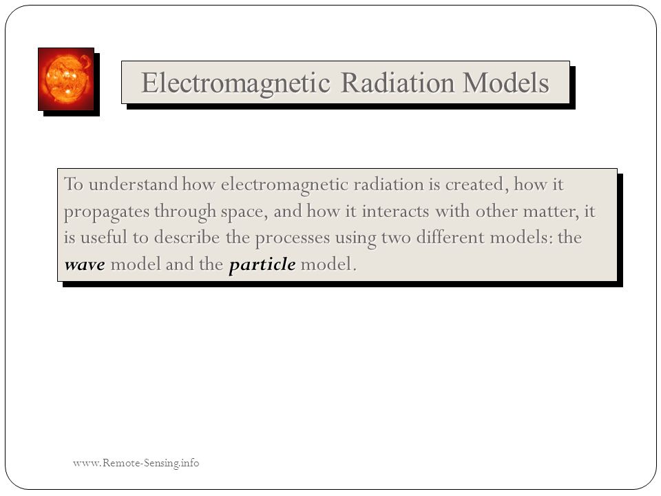
Electromagnetic Radiation Models To understand how electromagnetic radiation is created, how it propagates through space, and how it interacts with other matter, it is useful to describe the processes using two different models: the wave model and the particle model. www.Remote-Sensing.info
76
Wave Model of Electromagnetic Radiation In the 1860s, James Clerk Maxwell (1831–1879) conceptualized electromagnetic radiation (EMR) as an electromagnetic wave that travels through space at the speed of light, c, which is 3 x 10 8 meters per second (hereafter referred to as m s -1 ). The electromagnetic wave consists of two fluctuating fields—one electric and the other magnetic. The two vectors are at right angles (orthogonal) to one another, and both are perpendicular to the direction of travel. www.Remote-Sensing.info
 to one another, and both are perpendicular to the direction of travel.")
77
Radiometric Quantities The relationship between the wavelength ( ) and frequency ( ) of electromagnetic radiation is based on the following formula, where c is the speed of light: www.Remote-Sensing.info
 and frequency ( ) of electromagnetic radiation is based on the following formula, where c is the speed of light:")
78
Blackbody Radiation Curves Blackbody radiation curves for several objects including the Sun and the Earth which approximate 6,000 K and 300 K blackbodies, respectively. Blackbody radiation curves for several objects including the Sun and the Earth which approximate 6,000 K and 300 K blackbodies, respectively. The area under each curve may be summed to compute the total radiant energy (M ) exiting each object. Thus, the Sun produces more radiant exitance than the Earth because its temperature is greater. As the temperature of an object increases, its dominant wavelength ( max ) shifts toward the shorter wavelengths of the spectrum. www.Remote-Sensing.info
 exiting each object. Thus, the Sun produces more radiant exitance than the Earth because its temperature is greater. As the temperature of an object increases, its dominant wavelength ( max ) shifts toward the shorter wavelengths of the spectrum.")
79
Wein’s Displacement Law In addition to computing the total amount of energy exiting a theoretical blackbody such as the Sun, we can determine its dominant wavelength ( max ) based on Wien’s displacement law: where k is a constant equaling 2898 m K, and T is the absolute temperature in kelvin. Therefore, as the Sun approximates a 6000 K blackbody, its dominant wavelength ( max ) is 0.48 m: Where s is the Stefan-Boltzmann constant, 5.66697 x 10⁻⁸ W m-2 K-4. In addition to computing the total amount of energy exiting a theoretical blackbody such as the Sun, we can determine its dominant wavelength ( max ) based on Wien’s displacement law: where k is a constant equaling 2898 m K, and T is the absolute temperature in kelvin. Therefore, as the Sun approximates a 6000 K blackbody, its dominant wavelength ( max ) is 0.48 m: Where s is the Stefan-Boltzmann constant, 5.66697 x 10⁻⁸ W m-2 K-4. www.Remote-Sensing.info
 is 0.48 m: Where s is the Stefan-Boltzmann constant, x 10-8 W m-2 K-4. In addition to computing the total amount of energy exiting a theoretical blackbody such as the Sun, we can determine its dominant wavelength ( max ) based on Wien’s displacement law: where k is a constant equaling 2898 m K, and T is the absolute temperature in kelvin. Therefore, as the Sun approximates a 6000 K blackbody, its dominant wavelength ( max ) is 0.48 m: Where s is the Stefan-Boltzmann constant, x 10-8 W m-2 K-4.")
80
Radiometric Quantities All objects above absolute zero (–273°C or 0 K) emit electromagnetic energy, including water, soil, rock, vegetation, and the surface of the Sun. The Sun represents the initial source of most of the electromagnetic energy recorded by remote sensing systems (except RADAR, LIDAR, and SONAR). We may think of the Sun as a 5770 – 6,000 K blackbody (a theoretical construct that absorbs and radiates energy at the maximum possible rate per unit area at each wavelength ( ) for a given temperature). The total emitted radiation from a blackbody (M ) measured in watts per m -2 is proportional to the fourth power of its absolute temperature (T) measured in kelvin (K). This is known as the Stefan-Boltzmann law and is expressed as Where o is the Stefan-Boltzmann constant, 5.66697 x 10⁻⁸ W m-2 K-4. All objects above absolute zero (–273°C or 0 K) emit electromagnetic energy, including water, soil, rock, vegetation, and the surface of the Sun. The Sun represents the initial source of most of the electromagnetic energy recorded by remote sensing systems (except RADAR, LIDAR, and SONAR). We may think of the Sun as a 5770 – 6,000 K blackbody (a theoretical construct that absorbs and radiates energy at the maximum possible rate per unit area at each wavelength ( ) for a given temperature). The total emitted radiation from a blackbody (M ) measured in watts per m -2 is proportional to the fourth power of its absolute temperature (T) measured in kelvin (K). This is known as the Stefan-Boltzmann law and is expressed as Where o is the Stefan-Boltzmann constant, 5.66697 x 10⁻⁸ W m-2 K-4. www.Remote-Sensing.info
. We may think of the Sun as a 5770 – 6,000 K blackbody (a theoretical construct that absorbs and radiates energy at the maximum possible rate per unit area at each wavelength ( ) for a given temperature). The total emitted radiation from a blackbody (M ) measured in watts per m -2 is proportional to the fourth power of its absolute temperature (T) measured in kelvin (K). This is known as the Stefan-Boltzmann law and is expressed as Where o is the Stefan-Boltzmann constant, x 10-8 W m-2 K-4. All objects above absolute zero (–273°C or 0 K) emit electromagnetic energy, including water, soil, rock, vegetation, and the surface of the Sun. The Sun represents the initial source of most of the electromagnetic energy recorded by remote sensing systems (except RADAR, LIDAR, and SONAR). We may think of the Sun as a 5770 – 6,000 K blackbody (a theoretical construct that absorbs and radiates energy at the maximum possible rate per unit area at each wavelength ( ) for a given temperature). The total emitted radiation from a blackbody (M ) measured in watts per m -2 is proportional to the fourth power of its absolute temperature (T) measured in kelvin (K). This is known as the Stefan-Boltzmann law and is expressed as Where o is the Stefan-Boltzmann constant, x 10-8 W m-2 K-4.")
81
Creation of Light from Atomic Particles www.Remote-Sensing.info

82
Atmospheric Refraction Refraction in three nonturbulent atmospheric layers. The incident energy is bent from its normal trajectory as it travels from one atmospheric layer to another. Snell’s law can be used to predict how much bending will take place, based on a knowledge of the angle of incidence ( ) and the index of refraction of each atmospheric level, n 1, n 2, n 3. www.Remote-Sensing.info
 and the index of refraction of each atmospheric level, n 1, n 2, n 3.")
83
Snell’s Law Refraction can be described by Snell’s law, which states that for a given frequency of light (we must use frequency since, unlike wavelength, it does not change when the speed of light changes), the product of the index of refraction and the sine of the angle between the ray and a line normal to the interface is constant: From the accompanying figure, we can see that a nonturbulent atmosphere can be thought of as a series of layers of gases, each with a slightly different density. Anytime energy is propagated through the atmosphere for any appreciable distance at any angle other than vertical, refraction occurs. Refraction can be described by Snell’s law, which states that for a given frequency of light (we must use frequency since, unlike wavelength, it does not change when the speed of light changes), the product of the index of refraction and the sine of the angle between the ray and a line normal to the interface is constant: From the accompanying figure, we can see that a nonturbulent atmosphere can be thought of as a series of layers of gases, each with a slightly different density. Anytime energy is propagated through the atmosphere for any appreciable distance at any angle other than vertical, refraction occurs. www.Remote-Sensing.info
, the product of the index of refraction and the sine of the angle between the ray and a line normal to the interface is constant: From the accompanying figure, we can see that a nonturbulent atmosphere can be thought of as a series of layers of gases, each with a slightly different density. Anytime energy is propagated through the atmosphere for any appreciable distance at any angle other than vertical, refraction occurs.")
84
Atmospheric Scattering Type of scattering is a function of: 1)the wavelength of the incident radiant energy, and 2)the size of the gas molecule, dust particle, and/or water vapor droplet encountered. Type of scattering is a function of: 1)the wavelength of the incident radiant energy, and 2)the size of the gas molecule, dust particle, and/or water vapor droplet encountered. www.Remote-Sensing.info
the wavelength of the incident radiant energy, and 2)the size of the gas molecule, dust particle, and/or water vapor droplet encountered.")
85
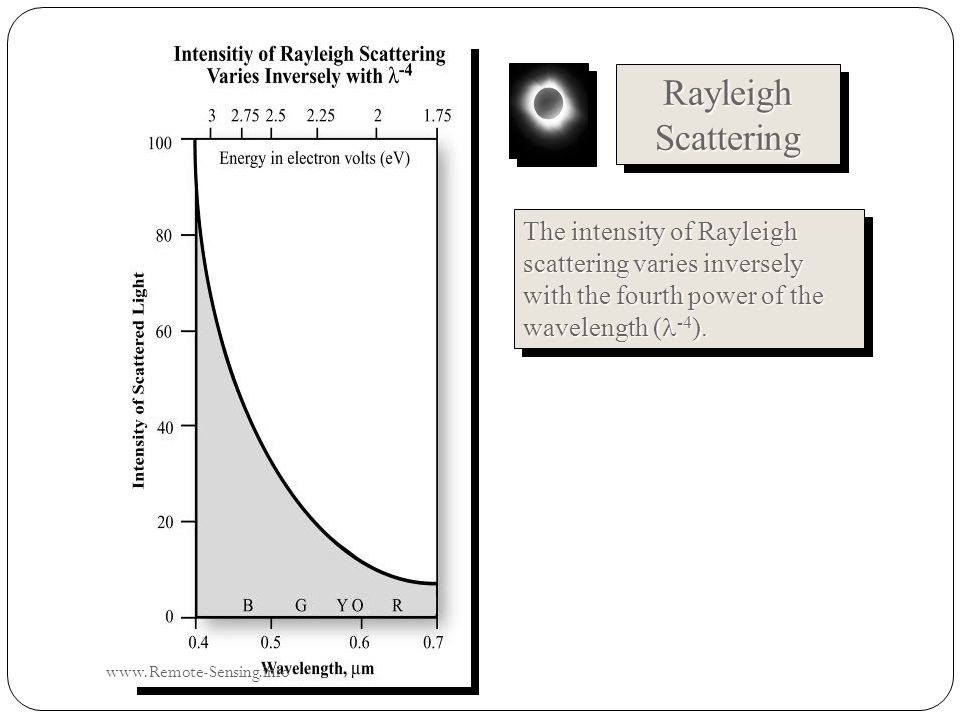
RayleighScatteringRayleighScattering The intensity of Rayleigh scattering varies inversely with the fourth power of the wavelength ( -4 ). www.Remote-Sensing.info
86
Absorption of the Sun's Incident Electromagnetic Energy in the Region from 0.1 to 30 m by Various Atmospheric Gases window www.Remote-Sensing.info

87
ReflectanceReflectance

88
Radiometric quantities have been identified that allow analysts to keep a careful record of the incident and exiting radiant flux. We begin with the simple radiation budget equation: Terrain Energy-Matter Interactions www.Remote-Sensing.info

89
Hemispherical Reflectance, Absorptance, and Transmittance The Hemispherical reflectance ( ) is defined as the dimensionless ratio of the radiant flux reflected from a surface to the radiant flux incident to it: Hemispherical transmittance ( ) is defined as the dimensionless ratio of the radiant flux transmitted through a surface to the radiant flux incident to it: Hemispherical absorptance ( ) is defined by the dimensionless relationship: The Hemispherical reflectance ( ) is defined as the dimensionless ratio of the radiant flux reflected from a surface to the radiant flux incident to it: Hemispherical transmittance ( ) is defined as the dimensionless ratio of the radiant flux transmitted through a surface to the radiant flux incident to it: Hemispherical absorptance ( ) is defined by the dimensionless relationship: www.Remote-Sensing.info
 is defined as the dimensionless ratio of the radiant flux reflected from a surface to the radiant flux incident to it: Hemispherical transmittance ( ) is defined as the dimensionless ratio of the radiant flux transmitted through a surface to the radiant flux incident to it: Hemispherical absorptance ( ) is defined by the dimensionless relationship: The Hemispherical reflectance ( ) is defined as the dimensionless ratio of the radiant flux reflected from a surface to the radiant flux incident to it: Hemispherical transmittance ( ) is defined as the dimensionless ratio of the radiant flux transmitted through a surface to the radiant flux incident to it: Hemispherical absorptance ( ) is defined by the dimensionless relationship:")
90
Correcting Remote Sensing System Detector Error Ideally, the radiance recorded by a remote sensing system in various bands is an accurate representation of the radiance actually leaving the feature of interest (e.g., soil, vegetation, water, or urban land cover) on the Earth’s surface. Unfortunately, noise (error) can enter the data-collection system at several points. For example, radiometric error in remotely sensed data may be introduced by the sensor system itself when the individual detectors do not function properly or are improperly calibrated. Several of the more common remote sensing system–induced radiometric errors are: random bad pixels (shot noise), random bad pixels (shot noise), line-start/stop problems, line-start/stop problems, line or column drop-outs, line or column drop-outs, partial line or column drop-outs, and partial line or column drop-outs, and line or column striping. line or column striping. Ideally, the radiance recorded by a remote sensing system in various bands is an accurate representation of the radiance actually leaving the feature of interest (e.g., soil, vegetation, water, or urban land cover) on the Earth’s surface. Unfortunately, noise (error) can enter the data-collection system at several points. For example, radiometric error in remotely sensed data may be introduced by the sensor system itself when the individual detectors do not function properly or are improperly calibrated. Several of the more common remote sensing system–induced radiometric errors are: random bad pixels (shot noise), random bad pixels (shot noise), line-start/stop problems, line-start/stop problems, line or column drop-outs, line or column drop-outs, partial line or column drop-outs, and partial line or column drop-outs, and line or column striping. line or column striping. www.Remote-Sensing.info
 can enter the data-collection system at several points. For example, radiometric error in remotely sensed data may be introduced by the sensor system itself when the individual detectors do not function properly or are improperly calibrated. Several of the more common remote sensing system–induced radiometric errors are: random bad pixels (shot noise), random bad pixels (shot noise), line-start/stop problems, line-start/stop problems, line or column drop-outs, line or column drop-outs, partial line or column drop-outs, and partial line or column drop-outs, and line or column striping. line or column striping. Ideally, the radiance recorded by a remote sensing system in various bands is an accurate representation of the radiance actually leaving the feature of interest (e.g., soil, vegetation, water, or urban land cover) on the Earth’s surface. Unfortunately, noise (error) can enter the data-collection system at several points. For example, radiometric error in remotely sensed data may be introduced by the sensor system itself when the individual detectors do not function properly or are improperly calibrated. Several of the more common remote sensing system–induced radiometric errors are: random bad pixels (shot noise), random bad pixels (shot noise), line-start/stop problems, line-start/stop problems, line or column drop-outs, line or column drop-outs, partial line or column drop-outs, and partial line or column drop-outs, and line or column striping. line or column striping.")
91
Random Bad Pixels (Shot Noise) The mean of the eight surrounding pixels is computed using the equation and the value substituted for BV i,j,k in the corrected image: www.Remote-Sensing.info
 The mean of the eight surrounding pixels is computed using the equation and the value substituted for BV i,j,k in the corrected image:")
92
Line or Column Drop-outs It is first necessary to locate each bad line in the dataset. A simple thresholding algorithm makes a pass through the dataset and flags any scan line having a mean brightness value at or near zero. Once identified, it is then possible to evaluate the output for a pixel in the preceding line (BV i – 1,j,k ) and succeeding line (BV i + 1,j,k ) and assign the output pixel (BV i,j,k ) in the drop-out line the average of these two brightness values: This is performed for every pixel in a bad scan line. The result is an image consisting of interpolated data every nth line that is more visually interpretable than one with horizontal black lines running systematically throughout the entire image. This same cosmetic digital image processing procedure can be applied to column drop-outs produced by a linear array remote sensing system. It is first necessary to locate each bad line in the dataset. A simple thresholding algorithm makes a pass through the dataset and flags any scan line having a mean brightness value at or near zero. Once identified, it is then possible to evaluate the output for a pixel in the preceding line (BV i – 1,j,k ) and succeeding line (BV i + 1,j,k ) and assign the output pixel (BV i,j,k ) in the drop-out line the average of these two brightness values: This is performed for every pixel in a bad scan line. The result is an image consisting of interpolated data every nth line that is more visually interpretable than one with horizontal black lines running systematically throughout the entire image. This same cosmetic digital image processing procedure can be applied to column drop-outs produced by a linear array remote sensing system. www.Remote-Sensing.info
 and succeeding line (BV i + 1,j,k ) and assign the output pixel (BV i,j,k ) in the drop-out line the average of these two brightness values: This is performed for every pixel in a bad scan line. The result is an image consisting of interpolated data every nth line that is more visually interpretable than one with horizontal black lines running systematically throughout the entire image. This same cosmetic digital image processing procedure can be applied to column drop-outs produced by a linear array remote sensing system. It is first necessary to locate each bad line in the dataset. A simple thresholding algorithm makes a pass through the dataset and flags any scan line having a mean brightness value at or near zero. Once identified, it is then possible to evaluate the output for a pixel in the preceding line (BV i – 1,j,k ) and succeeding line (BV i + 1,j,k ) and assign the output pixel (BV i,j,k ) in the drop-out line the average of these two brightness values: This is performed for every pixel in a bad scan line. The result is an image consisting of interpolated data every nth line that is more visually interpretable than one with horizontal black lines running systematically throughout the entire image. This same cosmetic digital image processing procedure can be applied to column drop-outs produced by a linear array remote sensing system.")
93
N-line Striping Sometimes a detector does not fail completely, but simply goes out of radiometric adjustment. For example, a detector might record spectral measurements over a dark, deep body of water that are almost uniformly 20 brightness values greater than the other detectors for the same band. The result would be an image with systematic, noticeable lines that are brighter than adjacent lines. This is referred to as. The maladjusted line contains valuable information, but should be corrected to have approximately the same radiometric scale as the data collected by the properly calibrated detectors associated with the same band. Sometimes a detector does not fail completely, but simply goes out of radiometric adjustment. For example, a detector might record spectral measurements over a dark, deep body of water that are almost uniformly 20 brightness values greater than the other detectors for the same band. The result would be an image with systematic, noticeable lines that are brighter than adjacent lines. This is referred to as n-line striping. The maladjusted line contains valuable information, but should be corrected to have approximately the same radiometric scale as the data collected by the properly calibrated detectors associated with the same band. To repair systematic n-line striping, it is first necessary to identify the miscalibrated scan lines in the scene. This is usually accomplished by computing a histogram of the values for each of the n detectors that collected data over the entire scene (ideally, this would take place over a homogeneous area, such as a body of water). If one detector’s mean or median is significantly different from the others, it is probable that this detector is out of adjustment. Consequently, every line and pixel in the scene recorded by the maladjusted detector may require a bias (additive or subtractive) correction or a more severe gain (multiplicative) correction. This type of n-line striping correction a) adjusts all the bad scan lines so that they have approximately the same radiometric scale as the correctly collected data and b) improves the visual interpretability of the data. It looks better. Sometimes a detector does not fail completely, but simply goes out of radiometric adjustment. For example, a detector might record spectral measurements over a dark, deep body of water that are almost uniformly 20 brightness values greater than the other detectors for the same band. The result would be an image with systematic, noticeable lines that are brighter than adjacent lines. This is referred to as. The maladjusted line contains valuable information, but should be corrected to have approximately the same radiometric scale as the data collected by the properly calibrated detectors associated with the same band. Sometimes a detector does not fail completely, but simply goes out of radiometric adjustment. For example, a detector might record spectral measurements over a dark, deep body of water that are almost uniformly 20 brightness values greater than the other detectors for the same band. The result would be an image with systematic, noticeable lines that are brighter than adjacent lines. This is referred to as n-line striping. The maladjusted line contains valuable information, but should be corrected to have approximately the same radiometric scale as the data collected by the properly calibrated detectors associated with the same band. To repair systematic n-line striping, it is first necessary to identify the miscalibrated scan lines in the scene. This is usually accomplished by computing a histogram of the values for each of the n detectors that collected data over the entire scene (ideally, this would take place over a homogeneous area, such as a body of water). If one detector’s mean or median is significantly different from the others, it is probable that this detector is out of adjustment. Consequently, every line and pixel in the scene recorded by the maladjusted detector may require a bias (additive or subtractive) correction or a more severe gain (multiplicative) correction. This type of n-line striping correction a) adjusts all the bad scan lines so that they have approximately the same radiometric scale as the correctly collected data and b) improves the visual interpretability of the data. It looks better. www.Remote-Sensing.info
. If one detector’s mean or median is significantly different from the others, it is probable that this detector is out of adjustment. Consequently, every line and pixel in the scene recorded by the maladjusted detector may require a bias (additive or subtractive) correction or a more severe gain (multiplicative) correction. This type of n-line striping correction a) adjusts all the bad scan lines so that they have approximately the same radiometric scale as the correctly collected data and b) improves the visual interpretability of the data. It looks better. Sometimes a detector does not fail completely, but simply goes out of radiometric adjustment. For example, a detector might record spectral measurements over a dark, deep body of water that are almost uniformly 20 brightness values greater than the other detectors for the same band. The result would be an image with systematic, noticeable lines that are brighter than adjacent lines. This is referred to as. The maladjusted line contains valuable information, but should be corrected to have approximately the same radiometric scale as the data collected by the properly calibrated detectors associated with the same band. Sometimes a detector does not fail completely, but simply goes out of radiometric adjustment. For example, a detector might record spectral measurements over a dark, deep body of water that are almost uniformly 20 brightness values greater than the other detectors for the same band. The result would be an image with systematic, noticeable lines that are brighter than adjacent lines. This is referred to as n-line striping. The maladjusted line contains valuable information, but should be corrected to have approximately the same radiometric scale as the data collected by the properly calibrated detectors associated with the same band. To repair systematic n-line striping, it is first necessary to identify the miscalibrated scan lines in the scene. This is usually accomplished by computing a histogram of the values for each of the n detectors that collected data over the entire scene (ideally, this would take place over a homogeneous area, such as a body of water). If one detector’s mean or median is significantly different from the others, it is probable that this detector is out of adjustment. Consequently, every line and pixel in the scene recorded by the maladjusted detector may require a bias (additive or subtractive) correction or a more severe gain (multiplicative) correction. This type of n-line striping correction a) adjusts all the bad scan lines so that they have approximately the same radiometric scale as the correctly collected data and b) improves the visual interpretability of the data. It looks better.")
94
Types of Atmospheric Correction There are several ways to atmospherically correct remotely sensed data. Some are relatively straightforward while others are complex, being founded on physical principles and requiring a significant amount of information to function properly. This discussion will focus on two major types of atmospheric correction: Absolute atmospheric correction, and Relative atmospheric correction. There are various methods that can be used to achieve absolute or relative atmospheric correction. The following sections identify the logic, algorithms, and problems associated with each methodology. There are several ways to atmospherically correct remotely sensed data. Some are relatively straightforward while others are complex, being founded on physical principles and requiring a significant amount of information to function properly. This discussion will focus on two major types of atmospheric correction: Absolute atmospheric correction, and Relative atmospheric correction. There are various methods that can be used to achieve absolute or relative atmospheric correction. The following sections identify the logic, algorithms, and problems associated with each methodology. www.Remote-Sensing.info

95
Absolute Atmospheric Correction Solar radiation is largely unaffected as it travels through the vacuum of space. When it interacts with the Earth’s atmosphere, however, it is selectively scattered and absorbed. The sum of these two forms of energy loss is called. Atmospheric attenuation may 1) make it difficult to relate hand-held in situ spectroradiometer measurements with remote measurements, 2) make it difficult to extend spectral signatures through space and time, and (3) have an impact on classification accuracy within a scene if atmospheric attenuation varies significantly throughout the image. Solar radiation is largely unaffected as it travels through the vacuum of space. When it interacts with the Earth’s atmosphere, however, it is selectively scattered and absorbed. The sum of these two forms of energy loss is called atmospheric attenuation. Atmospheric attenuation may 1) make it difficult to relate hand-held in situ spectroradiometer measurements with remote measurements, 2) make it difficult to extend spectral signatures through space and time, and (3) have an impact on classification accuracy within a scene if atmospheric attenuation varies significantly throughout the image. The general goal of absolute radiometric correction is to turn the digital brightness values recorded by a remote sensing system into values. These values can then be compared or used in conjunction with scaled surface reflectance values obtained anywhere else on the planet. The general goal of absolute radiometric correction is to turn the digital brightness values recorded by a remote sensing system into scaled surface reflectance values. These values can then be compared or used in conjunction with scaled surface reflectance values obtained anywhere else on the planet. Solar radiation is largely unaffected as it travels through the vacuum of space. When it interacts with the Earth’s atmosphere, however, it is selectively scattered and absorbed. The sum of these two forms of energy loss is called. Atmospheric attenuation may 1) make it difficult to relate hand-held in situ spectroradiometer measurements with remote measurements, 2) make it difficult to extend spectral signatures through space and time, and (3) have an impact on classification accuracy within a scene if atmospheric attenuation varies significantly throughout the image. Solar radiation is largely unaffected as it travels through the vacuum of space. When it interacts with the Earth’s atmosphere, however, it is selectively scattered and absorbed. The sum of these two forms of energy loss is called atmospheric attenuation. Atmospheric attenuation may 1) make it difficult to relate hand-held in situ spectroradiometer measurements with remote measurements, 2) make it difficult to extend spectral signatures through space and time, and (3) have an impact on classification accuracy within a scene if atmospheric attenuation varies significantly throughout the image. The general goal of absolute radiometric correction is to turn the digital brightness values recorded by a remote sensing system into values. These values can then be compared or used in conjunction with scaled surface reflectance values obtained anywhere else on the planet. The general goal of absolute radiometric correction is to turn the digital brightness values recorded by a remote sensing system into scaled surface reflectance values. These values can then be compared or used in conjunction with scaled surface reflectance values obtained anywhere else on the planet. www.Remote-Sensing.info
 make it difficult to relate hand-held in situ spectroradiometer measurements with remote measurements, 2) make it difficult to extend spectral signatures through space and time, and (3) have an impact on classification accuracy within a scene if atmospheric attenuation varies significantly throughout the image. Solar radiation is largely unaffected as it travels through the vacuum of space. When it interacts with the Earth’s atmosphere, however, it is selectively scattered and absorbed. The sum of these two forms of energy loss is called atmospheric attenuation. Atmospheric attenuation may 1) make it difficult to relate hand-held in situ spectroradiometer measurements with remote measurements, 2) make it difficult to extend spectral signatures through space and time, and (3) have an impact on classification accuracy within a scene if atmospheric attenuation varies significantly throughout the image. The general goal of absolute radiometric correction is to turn the digital brightness values recorded by a remote sensing system into values. These values can then be compared or used in conjunction with scaled surface reflectance values obtained anywhere else on the planet. The general goal of absolute radiometric correction is to turn the digital brightness values recorded by a remote sensing system into scaled surface reflectance values. These values can then be compared or used in conjunction with scaled surface reflectance values obtained anywhere else on the planet. Solar radiation is largely unaffected as it travels through the vacuum of space. When it interacts with the Earth’s atmosphere, however, it is selectively scattered and absorbed. The sum of these two forms of energy loss is called. Atmospheric attenuation may 1) make it difficult to relate hand-held in situ spectroradiometer measurements with remote measurements, 2) make it difficult to extend spectral signatures through space and time, and (3) have an impact on classification accuracy within a scene if atmospheric attenuation varies significantly throughout the image. Solar radiation is largely unaffected as it travels through the vacuum of space. When it interacts with the Earth’s atmosphere, however, it is selectively scattered and absorbed. The sum of these two forms of energy loss is called atmospheric attenuation. Atmospheric attenuation may 1) make it difficult to relate hand-held in situ spectroradiometer measurements with remote measurements, 2) make it difficult to extend spectral signatures through space and time, and (3) have an impact on classification accuracy within a scene if atmospheric attenuation varies significantly throughout the image. The general goal of absolute radiometric correction is to turn the digital brightness values recorded by a remote sensing system into values. These values can then be compared or used in conjunction with scaled surface reflectance values obtained anywhere else on the planet. The general goal of absolute radiometric correction is to turn the digital brightness values recorded by a remote sensing system into scaled surface reflectance values. These values can then be compared or used in conjunction with scaled surface reflectance values obtained anywhere else on the planet.")
96
Absolute Atmospheric Correction Much research has been carried out to address the problem of correcting images for atmospheric effects. These efforts have resulted in a number of atmospheric radiative transfer codes (models) that can provide realistic estimates of the effects of atmospheric scattering and absorption on satellite imagery. Once these effects have been identified for a specific date of imagery, each band and/or pixel in the scene can be adjusted to remove the effects of scattering and/or absorption. The image is then considered to be atmospherically corrected. Unfortunately, the application of these codes to a specific scene and date also requires knowledge of both the sensor spectral profile and the atmospheric properties at the same time. Atmospheric properties are difficult to acquire even when planned. For most historic satellite data, they are not available. Even today, accurate scaled surface reflectance retrieval is not operational for the majority of satellite image sources used for land-cover change detection. An exception is NASA's Moderate Resolution Imaging Spectroradiometer (MODIS), for which surface reflectance products are available. Nevertheless, we will proceed with a general discussion of the important issues associated with absolute atmospheric correction and then provide examples of how absolute radiometric correction is performed. Much research has been carried out to address the problem of correcting images for atmospheric effects. These efforts have resulted in a number of atmospheric radiative transfer codes (models) that can provide realistic estimates of the effects of atmospheric scattering and absorption on satellite imagery. Once these effects have been identified for a specific date of imagery, each band and/or pixel in the scene can be adjusted to remove the effects of scattering and/or absorption. The image is then considered to be atmospherically corrected. Unfortunately, the application of these codes to a specific scene and date also requires knowledge of both the sensor spectral profile and the atmospheric properties at the same time. Atmospheric properties are difficult to acquire even when planned. For most historic satellite data, they are not available. Even today, accurate scaled surface reflectance retrieval is not operational for the majority of satellite image sources used for land-cover change detection. An exception is NASA's Moderate Resolution Imaging Spectroradiometer (MODIS), for which surface reflectance products are available. Nevertheless, we will proceed with a general discussion of the important issues associated with absolute atmospheric correction and then provide examples of how absolute radiometric correction is performed. www.Remote-Sensing.info
 that can provide realistic estimates of the effects of atmospheric scattering and absorption on satellite imagery. Once these effects have been identified for a specific date of imagery, each band and/or pixel in the scene can be adjusted to remove the effects of scattering and/or absorption. The image is then considered to be atmospherically corrected. Unfortunately, the application of these codes to a specific scene and date also requires knowledge of both the sensor spectral profile and the atmospheric properties at the same time. Atmospheric properties are difficult to acquire even when planned. For most historic satellite data, they are not available. Even today, accurate scaled surface reflectance retrieval is not operational for the majority of satellite image sources used for land-cover change detection. An exception is NASA s Moderate Resolution Imaging Spectroradiometer (MODIS), for which surface reflectance products are available. Nevertheless, we will proceed with a general discussion of the important issues associated with absolute atmospheric correction and then provide examples of how absolute radiometric correction is performed. Much research has been carried out to address the problem of correcting images for atmospheric effects. These efforts have resulted in a number of atmospheric radiative transfer codes (models) that can provide realistic estimates of the effects of atmospheric scattering and absorption on satellite imagery. Once these effects have been identified for a specific date of imagery, each band and/or pixel in the scene can be adjusted to remove the effects of scattering and/or absorption. The image is then considered to be atmospherically corrected. Unfortunately, the application of these codes to a specific scene and date also requires knowledge of both the sensor spectral profile and the atmospheric properties at the same time. Atmospheric properties are difficult to acquire even when planned. For most historic satellite data, they are not available. Even today, accurate scaled surface reflectance retrieval is not operational for the majority of satellite image sources used for land-cover change detection. An exception is NASA s Moderate Resolution Imaging Spectroradiometer (MODIS), for which surface reflectance products are available. Nevertheless, we will proceed with a general discussion of the important issues associated with absolute atmospheric correction and then provide examples of how absolute radiometric correction is performed.")
97
Radiance (L T ) from paths 1, 3, and 5 contains intrinsic valuable spectral information about the target of interest. Conversely, the path radiance (L p ) from paths 2 and 4 includes diffuse sky irradiance or radiance from neighboring areas on the ground. This path radiance generally introduces unwanted radiometric noise in the remotely sensed data and complicates the image interpretation process. www.Remote-Sensing.info
 from paths 2 and 4 includes diffuse sky irradiance or radiance from neighboring areas on the ground. This path radiance generally introduces unwanted radiometric noise in the remotely sensed data and complicates the image interpretation process.")
98
The total radiance reaching the sensor is: This may be summarized as: www.Remote-Sensing.info

99
Radiometric Correction Using Empirical Line Calibration Radiometric Correction Using Empirical Line Calibration Absolute atmospheric correction may also be performed using empirical line calibration (ELC), which forces the remote sensing image data to match in situ spectral reflectance measurements, hopefully obtained at approximately the same time and on the same date as the remote sensing overflight. Empirical line calibration is based on the equation: where BV k is the digital output value for a pixel in band k, p equals the scaled surface reflectance of the materials within the remote sensor IFOV at a specific wavelength ( ), A k is a multiplicative term affecting the BV, and B k is an additive term. The multiplicative term is associated primarily with atmospheric transmittance and instrumental factors, and the additive term deals primarily with atmospheric path radiance and instrumental offset (i.e., dark current). www.Remote-Sensing.info
, A k is a multiplicative term affecting the BV, and B k is an additive term. The multiplicative term is associated primarily with atmospheric transmittance and instrumental factors, and the additive term deals primarily with atmospheric path radiance and instrumental offset (i.e., dark current).")
100
Field spectra Band 1 Band 2 Band 3 One Bright Target 4849 4847 5048 5554 5754 5655 4040 3940 4142 Radiance image (e.g., Band 1) Band 1 Band 2 Band 3 One Dark Target 910 1110 1012 54 56 64 00 40 12 Wavelength, nm Radiance Field spectra Paired Relationship: Band 1 Band 2 Band 3 DarkTarget DarkTarget BrightTarget BrightTarget Remotemeasurement Field spectra = 55 Remote Measurement = 49 = 55 F = 59 = 41 F = 48 Field spectra = 13 Remote Measurement = 11 = 5 F = 7 = 3 F = 4 www.Remote-Sensing.info
 Band 1 Band 2 Band 3 One Dark Target Wavelength, nm Radiance Field spectra Paired Relationship: Band 1 Band 2 Band 3 DarkTarget DarkTarget BrightTarget BrightTarget Remotemeasurement Field spectra = 55 Remote Measurement = 49 = 55 F = 59 = 41 F = 48 Field spectra = 13 Remote Measurement = 11 = 5 F = 7 = 3 F = 4")
101
Cosine Correction for Terrain Slope Cosine Correction for Terrain Slope where: L H = radiance observed for a horizontal surface (i.e., slope-aspect corrected surface (i.e., slope-aspect corrected remote sensor data). remote sensor data). L T = radiance observed over sloped terrain (i.e., the raw remote sensor data) (i.e., the raw remote sensor data) 0 = sun’s zenith angle i = sun’s incidence angle in relation to the i = sun’s incidence angle in relation to the normal on a pixel normal on a pixelwhere: L H = radiance observed for a horizontal surface (i.e., slope-aspect corrected surface (i.e., slope-aspect corrected remote sensor data). remote sensor data). L T = radiance observed over sloped terrain (i.e., the raw remote sensor data) (i.e., the raw remote sensor data) 0 = sun’s zenith angle i = sun’s incidence angle in relation to the i = sun’s incidence angle in relation to the normal on a pixel normal on a pixel www.Remote-Sensing.info
. L T = radiance observed over sloped terrain (i.e., the raw remote sensor data) (i.e., the raw remote sensor data) 0 = sun’s zenith angle i = sun’s incidence angle in relation to the i = sun’s incidence angle in relation to the normal on a pixel normal on a pixelwhere: L H = radiance observed for a horizontal surface (i.e., slope-aspect corrected surface (i.e., slope-aspect corrected remote sensor data). remote sensor data). L T = radiance observed over sloped terrain (i.e., the raw remote sensor data) (i.e., the raw remote sensor data) 0 = sun’s zenith angle i = sun’s incidence angle in relation to the i = sun’s incidence angle in relation to the normal on a pixel normal on a pixel")
Similar presentations

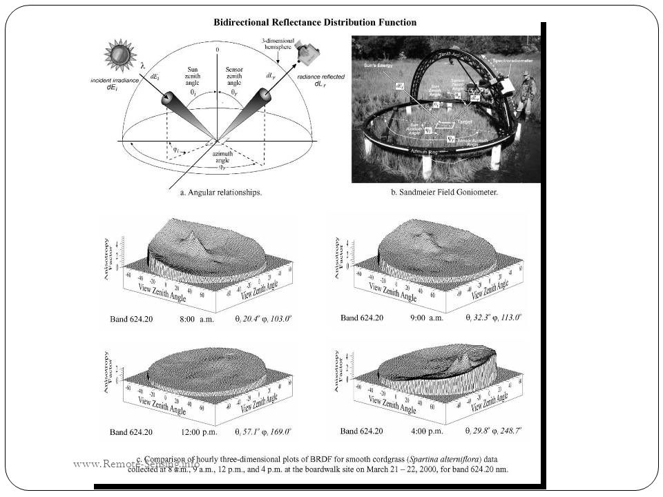
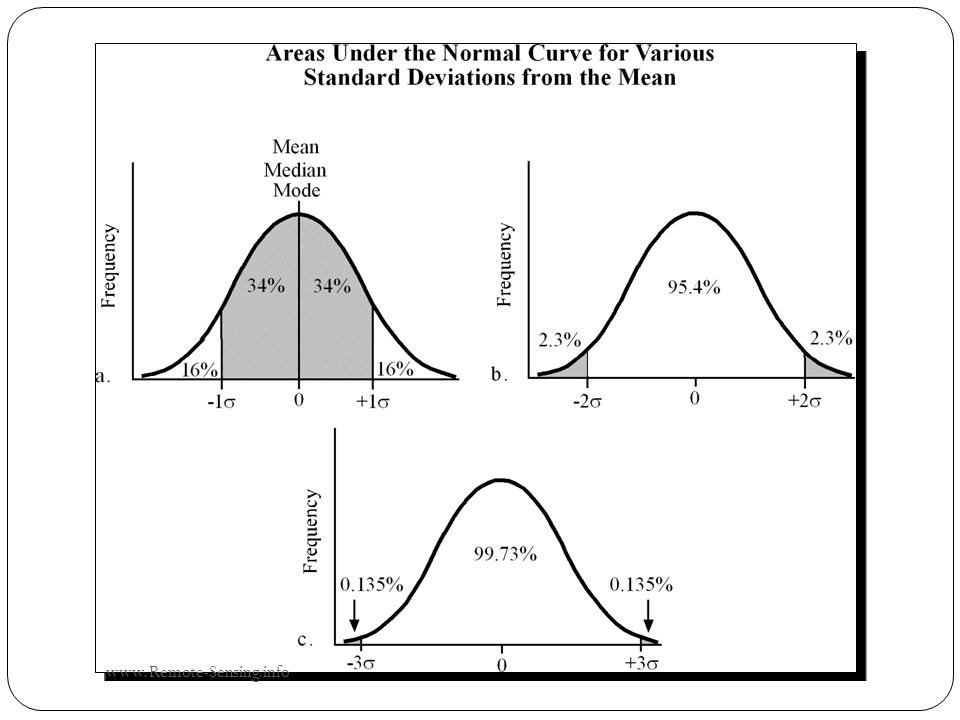


 Image Quality Assessment Radiometric Correction Geometric Correction Image Classification Introduction.>")


>")


