1. Chapter 8 PD-Method and Local Ratio (5) Equivalence This ppt is editored from a ppt of Reuven Bar-Yehuda. Reuven Bar-Yehuda

2. 2 Introduction The local ratio technique is an approximation paradigm for NP-hard optimization to obtain approximate solutions Its main feature of attraction is its simplicity and elegance; it is very easy to understand, and has surprisingly broad applicability.

3. 3 A Vertex Cover Problem: Network Testing A network tester involves placing probes onto the network vertices. A probe can determine if a connected link is working correctly. The goal is to minimize the number of used probes to check all the links.

4. 4 A Vertex Cover Problem: Precedence Constrained Scheduling Schedule a set of jobs on a single machine; Jobs have precedence constraints between them; The goal is to find a schedule which minimizes the weighted sum of completion times. This problem can be formulated as a vertex cover problem [Ambuehl- Mastrolilli’05]

5. 5 The Local Ratio Theorem (for minimization problems) Let w = w 1 + w 2. If x is an r-approximate solution for w 1 and w 2 then x is r- approximate with respect to w as well. Note that the theorem holds even when negative weights are allowed. Proof

6. 6 Vertex Cover example W = [41, 62, 13, 14, 35, 26, 17] W 1 = [ 0, 0, 0, 14, 14, 0, 0] W 2 = [41, 62, 13, 0, 21, 26, 17] W = W 1 + W 2 Weight functions: 4141 62 1414 35 17 26 13

7. 7 Vertex Cover example (step 1) =+ 4141 62 1414 35 17 26 13 0 0 1414 14 0 0 0 4141 62 0 21 17 26 13 Note: any feasible solution is a 2-approximate solution for weight function W 1

8. 8 Vertex Cover example (step 2) =+ 4141 62 0 21 17 26 13 0 0 0 21 0 0 4141 62 0 0 17 5 13

9. 9 Vertex Cover example (step 3) =+ 4141 62 0 0 17 5 13 4141 41 0 0 0 0 0 0 21 0 0 17 5 13

10. 10 Vertex Cover example (step 4) =+ 0 21 0 0 17 5 13 0 0 0 0 0 0 8 0 0 17 5 0

11. 11 Vertex Cover example (step 5) =+ 0 8 0 0 17 5 0 0 8 0 0 12 0 0 0 0 0 0 5 5 0

12. Vertex Cover example (step 6) The optimal solution value of the VC instance on the left is zero. By a recurrent application of the Local Ratio Theorem we are guaranteed to be within 2 times the optimal solution value by picking the zero nodes. Opt = 120 Approx = 129 0 8 0 0 12 0 0 416213 14 35 26 17

13. 13 1. For each edge {u,v} do: 2. Let  = min {w(u), w(v)}. 3. w(u)  w(u) - . 4. w(v)  w(v) - . 5. Return {v | w(v) = 0}. 2-Approx VC (Bar-Yehuda & Even 81) Iterative implementation – edge by edge

14. 14 Recursive implementation 1.If a zero-cost solution can be found, return one. 2.Otherwise, find a suitable decomposition of w into two weight functions w 1 and w 2 = w − w 1, and solve the problem recursively, using w 2 as the weight function in the recursive call. The Local Ratio Theorem leads naturally to the formulation of recursive algorithms with the following general structure

15. 15 2-Approx VC (Bar-Yehuda & Even 81) Recursive implementation – edge by edge 1.VC (V, E, w) 2.If E=  return  ; 3.If  w(v)=0 return {v}+VC(V-{v}, E-E(v), w); 4.Let (x,y)  E; 5.Let  = min{p(x), p(y)}; 6.Define w 1 (v) =  if v=x or v=y and 0 otherwise; 7.Return VC(V, E, w- w 1 )

16. 16 Algorithm Analysis We prove that the solution returned by the algorithm is 2- approximate by induction on the recursion and by using the Local Ratio Theorem. 1.In the base case, the algorithm returns a vertex cover of zero cost, which is optimal. 2.For the inductive step, consider the solution returned by the recursive call. By the inductive hypothesis it is 2-approximate with respect to w 2. We claim that it is also 2-approximate with respect to w 1. In fact, every feasible solution is 2-approximate with respect to w 1.

17. 17 Generality of the analysis The proof that a given algorithm is an r- approximation algorithm is by induction on the recursion. In the base case, the solution is optimal (and, therefore, r-approximate) because it has zero cost, and in the inductive step, the solution returned by the recursive call is r-approximate with respect to w 2 by the inductive hypothesis. Thus, different algorithms differ from one another only in the choice of w 1, and in the proof that every feasible solution is r-approximate with respect to w 1.Thus, different algorithms differ from one another only in the choice of w 1, and in the proof that every feasible solution is r-approximate with respect to w 1.

18. 18 The key ingredient Different algorithms (for different problems), differ from one another only in the decomposition of W, and this decomposition is determined completely by the choice of W 1. W 2 = W – W 1

19. 19 The creative part… find r-effective weights w 1 is fully r-effective if there exists a number b such that b  w 1 · x  r · b for all feasible solutions x

20. 20 Framework Proving this amounts to proving that: 1.b is a lower bound on the optimum value, 2.r ·b is an upper bound on the cost of every feasible solution …and thus every feasible solution is r- approximate (all with respect to w 1 ). The analysis of algorithms in our framework boils down to proving that w 1 is r-effective.

23. 23 A different W 1 for VC star by star (Clarkson’83) 4141 62 1616 35 17 26 13 L e t x 2 V w i t h m i n i mum" = w ( x ) d ( x ) 16/ 4 1616 0 0 3737 58 031 13 26 13 =+ Let d(x) be the degree of vertex x

24. 24 A different W 1 for VC star by star L e t x 2 V w i t h m i n i mum" = w ( x ) d ( x )   44   0 0 b = 4 ·  is a lower bound on the optimum value, 2 ·b is an upper bound on the cost of every feasible solution W 1 is 2-effective

25. 25 Another W 1 for VC homogeneous (= proportional to the potential coverage) L e t " = m i n x 2 V w ( x ) d ( x ) 3  4  44 5  3  2  b = |E| ·  is a lower bound on the optimum value, 2 ·b is an upper bound on the cost of every feasible solution W 1 is 2-effective

28. 28 Partial Vertex Cover Input: VC with a fixed number k Goal: Identify a minimum cost subset of vertices that hits at least k edges Examples: if k = 1 then OPT = 13 if k = 3 then OPT = 14 if k = 5 then OPT = 25 if k = 6 then OPT = 14+13 4141 62 1414 25 17 26 13

29. 29 w=[41, 62, 13, 14, 25, 26, 17] w 1 =[ 0, 0, 0, 14, 14, 0, 0] w 2 =[41, 62, 13, 0, 11, 26, 17] w = w 1 + w 2 Weight functions: Assume k < |E| (number of edges) Note: NOT every feasible solution is a 2-approximate solution for weight function w 1 In VC every edge must be hit by a vertex. In partial VC, k vertices are sufficient. So the optimum for w 1 is 0 (k<=5); vice versa the solution that takes for example vertex 4 is infinite many times larger than the optimum 4141 62 1414 25 17 26 13 Partial Vertex Cover }

30. 30 Positive Weight Function We do not know of any single subset that must contribute to all solutions. To prevent OPT from being equal to 0, we can assign a positive weight to every element.

31. 31 w=[41, 62, 13, 14, 25, 26, 17] w 1 =[ 0, 0, 0, 14, 14, 0, 0] w 2 =[41, 62, 13, 0, 11, 26, 17] w = w 1 + w 2 Weight functions: Observe that 14 is NOT a lower bound of the optimal value! For example for k=1 then 13 is the optimal value. 4141 62 1414 25 17 26 13 Positive Weight Function

32. 32 x Let d(x) be the degree of vertex x What is the amortized cost to hit one edge by using x ? What is the minimal amortized cost to hit any edge? Positive Weight Function

33. 33 Positive Weight Function W 1 w 1 (x) =  · min{ d(x), k } For k = 3 then  = 14/3 Weight functions (k=3): w = [41, 62, 13, 14, 25, 26, 17] w 1 = [14, 14, 28/3, 14, 14, 14, 14] w 2 = [27, 48, 11/3, 0, 11, 12, 3] w = w 1 + w 2 4141 62 1414 25 17 26 13

34. 34 Function W 1 [Lower Bound] Every feasible solution costs at least  k = 14 [Upper Bound] There are feasible solutions whose value can be arbitrarily larger than  k (e.g. take all the vertices) But if you take all the vertices then not all of them are strictly necessary!! We can focus on Minimal Solutions!!! 1414 14 1414 28/3

35. 35 Minimal Solutions By minimal solution we mean a feasible solution that is minimal with respect to set inclusion, that is, a feasible solution whose proper subsets are all infeasible. Minimal solutions are meaningful mainly in the context of covering problems (covering problems are problems for which feasible solutions are monotone inclusion-wise, that is, if a set X is a feasible solution, then so is every superset of X; MST is not a covering problem).

36. 36 Minimal Solutions: r-effective weights w 1 is r-effective if there exists a number b such that b  w 1 · x  r · b for all minimal feasible solution x

37. 37 The creative part… again find r-effective weights If we can show that our algorithm uses an r-effective w 1 and returns minimal solutions, we will have essentially proved that it is an r-approximation algorithm. Designing an algorithm to return minimal solutions is quite easy. Most of the creative effort is therefore expended in finding an r-effective weight function (for a small r).

38. 38 2-effective weight function 1.In terms of w 1 every feasible solution costs at least  · k 2.In terms of w 1 every minimal feasible solution costs at most 2 ·  · k Minimal solution = any proper subset is not a feasible solution

39. 39 Proof of 2. (= costs at most 2 ·  · k )

40. 40 Proof of 2. (cont.) x d 1 (x) = 2 d 2 (x) = 3

41. 41 The approximation algorithm L e t C b e t h ese t o f e d gesan d S ( x ) b e t h ese t o f e d ges t h a t are h i t b yx Algorithm from Bar-Yehuda et al. “Local Ratio: A Unified Framework for Approximation Algorithms” ACM Computing Surveys, 2004

42. 42 Algorithm Framework 1.If a zero-cost minimal solution can be found, do: optimal solution. 2.Otherwise, if the problem contains a zero-cost element, do: problem size reduction. 3.Otherwise, do: weight decomposition.

43. Partial Vertex Cover

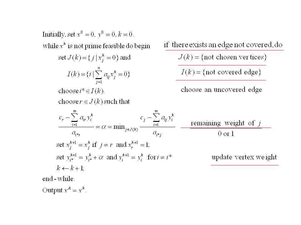
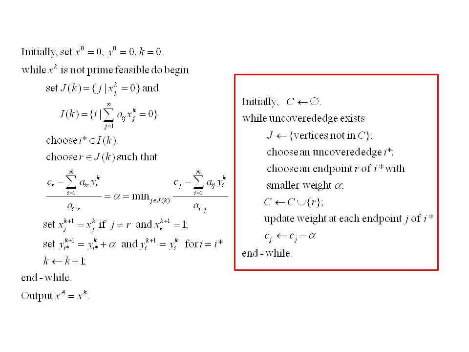
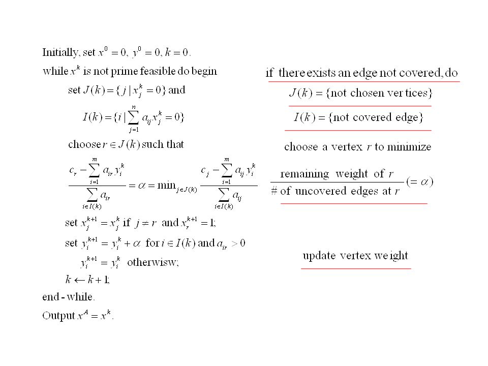
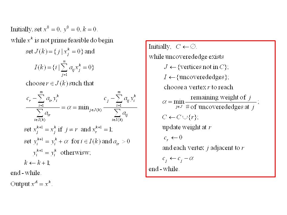
44. Primal and Dual

45. Complementary Slackness Condition primal dual

46. Complementary Slackness Condition primal dual

47. Primal-Dual schema ???