2. A general approximation technique for constrained forest problems Michael X. Goemans & David P. Williamson Presented by: Yonatan Elhanani & Yuval Cohen

3. Lecture Schedule Problem Description and Motivation Short Break Primal Dual (2-E)-Approximation

4. Forest Problems

5. Input is an undirected connected graph Output is a subgraph satisfying some condition. Our goal is to find the minimum weight feasible output (which is in fact a forest).

6. Some Interesting Problems Path between two vertices

7. Spanning Tree Steiner Tree Steiner Forest

8. Perfect Matching

9. T-join

10. Point to point connection

11. A General Framework Looking for a problem that generalizes all of the above, and possibly more. This way we can reduce the above to this problem and keep the approximation ratio.

12. Constrained Forest Problem

13. Input: The graph: Cost Function: Constraint Function: Output: A subset such that for each cut, that satisfies, holds.

14. Constrained Forest Problem We try to find…. Minimum Cut Cover (which is always A forest)

15. We will assume the following properties for : Symmetry: For each,. Satisfiability: Disjointness: If and then

16. The Meaning of epsilon Now we can state what the E is, for our (2-E)- approximation. Consider the set: Then, E=

17. Reductions to CFP We need the constraint functions.

18. Shortest Path Problem

19. Steiner Tree

20. Spanning Tree

21. Generalized Steiner Tree

22. Shortest Path (again)

23. T-Join

24. Minimum (Metric, Complete) Matching

25. Shortest Path (LAST TIME!)

26. Point to point Matching

27. Observation We notice that our problems are “connectivity” related, and that using our cuts, we inductively find these connections. Our algorithm will use a similar method, but with an optimal ratio guarantee.

28. We will resume in 10 minutes…

29. A (2-E)-Approximation algorithm In each step, this algorithm will greedily take the most cost effective edge that helps us satisfy an uncovered cut. Using the Primal Dual scheme we will prove the approximation ratio.

30. Definitions Let, be a component. is active [Inactive] if

31. The Formal Algorithm Input: An undirected graph, edge costs and a proper function Output: A forest and a value. 1. 2. (Implicitly sets ) 3. 4. For each 5. While 5.1. Find edge with,, that minimizes: 5.2. 5.3.For all with do 5.4. (Implicitly sets with ) 5.5. 6. For some connected component

32. Example We will observe an example of a simplified algorithm in order to get a better idea of how the algorithm works.

33. Example s,t in V. Algorithm for ants: 1.Initialize a component for each vertex. 2.While an active component exists: 2.1.“Expand” all active components until “impact”. 2.2.Unite colliding components. 2.3.Add the connecting edge to the solution. 3.Minimize solution.

34. Example s,t in V. Algorithm for ants: 1.Initialize a component for each vertex. 2.While an active component exists: 2.1.“Expand” all active components until “impact”. 2.2.Unite colliding components. 2.3.Add the connecting edge to the solution. 3.Minimize solution.

35. Example s,t in V. Algorithm for ants: 1.Initialize a component for each vertex. 2.While an active component exists: 2.1.”Expand” all active components until “impact”. 2.2.Unite colliding components. 2.3.Add the connecting edge to the solution. 3.Minimize solution.

36. Example s,t in V. Algorithm for ants: 1.Initialize a component for each vertex. 2.While an active component exists: 2.1.“Expand” all active components until “impact”. 2.2.Unite colliding components. 2.3.Add the connecting edge to the solution. 3.Minimize solution.

37. Example s,t in V. Algorithm for ants: 1.Initialize a component for each vertex. 2.While an active component exists: 2.1.“Expand” all active components until “impact”. 2.2.Unite colliding components. 2.3.Add the connecting edge to the solution. 3.Minimize solution.

38. Example s,t in V. Algorithm for ants: 1.Initialize a component for each vertex. 2.While an active component exists: 2.1.“Expand” all active components until “impact”. 2.2.Unite colliding components. 2.3.Add the connecting edge to the solution. 3.Minimize solution.

39. Example s,t in V. Algorithm for ants: 1.Initialize a component for each vertex. 2.While an active component exists: 2.1.“Expand” all active components until “impact”. 2.2.Unite colliding components. 2.3.Add the connecting edge to the solution. 3.Minimize solution.

40. Example s,t in V. Algorithm for ants: 1.Initialize a component for each vertex. 2.While an active component exists: 2.1.“Expand” all active components until “impact”. 2.2.Unite colliding components. 2.3.Add the connecting edge to the solution. 3.Minimize solution.

41. Example s,t in V. Algorithm for ants: 1.Initialize a component for each vertex. 2.While an active component exists: 2.1.“Expand” all active components until “impact”. 2.2.Unite colliding components. 2.3.Add the connecting edge to the solution. 3.Minimize solution.

42. Example s,t in V. Algorithm for ants: 1.Initialize a component for each vertex. 2.While an active component exists: 2.1.“Expand” all active components until “impact”. 2.2.Unite colliding components. 2.3.Add the connecting edge to the solution. 3.Minimize solution.

43. Example s,t in V. Algorithm for ants: 1.Initialize a component for each vertex. 2.While an active component exists: 2.1.“Expand” all active components until “impact”. 2.2.Unite colliding components. 2.3.Add the connecting edge to the solution. 3.Minimize solution.

44. Example s,t in V. Algorithm for ants: 1.Initialize a component for each vertex. 2.While an active component exists: 2.1.“Expand” all active components until “impact”. 2.2.Unite colliding components. 2.3.Add the connecting edge to the solution. 3.Minimize solution.

45. Example s,t in V. Algorithm for ants: 1.Initialize a component for each vertex. 2.While an active component exists: 2.1.“Expand” all active components until “impact”. 2.2.Unite colliding components. 2.3.Add the connecting edge to the solution. 3.Minimize solution.

46. Example s,t in V. Algorithm for ants: 1.Initialize a component for each vertex. 2.While an active component exists: 2.1.“Expand” all active components until “impact”. 2.2.Unite colliding components. 2.3.Add the connecting edge to the solution. 3.Minimize solution.

47. Example s,t in V. Algorithm for ants: 1.Initialize a component for each vertex. 2.While an active component exists: 2.1.“Expand” all active components until “impact”. 2.2.Unite colliding components. 2.3.Add the connecting edge to the solution. 3.Minimize solution.

48. Example s,t in V. Algorithm for ants: 1.Initialize a component for each vertex. 2.While an active component exists: 2.1.“Expand” all active components until “impact”. 2.2.Unite colliding components. 2.3.Add the connecting edge to the solution. 3.Minimize solution.

49. Example s,t in V. Algorithm for ants: 1.Initialize a component for each vertex. 2.While an active component exists: 2.1.“Expand” all active components until “impact”. 2.2.Unite colliding components. 2.3.Add the connecting edge to the solution. 3.Minimize solution.

50. Example s,t in V. Algorithm for ants: 1.Initialize a component for each vertex. 2.While an active component exists: 2.1.“Expand” all active components until “impact”. 2.2.Unite colliding components. 2.3.Add the connecting edge to the solution. 3.Minimize solution.

51. Example s,t in V. Algorithm for ants: 1.Initialize a component for each vertex. 2.While an active component exists: 2.1.“Expand” all active components until “impact”. 2.2.Unite colliding components. 2.3.Add the connecting edge to the solution. 3.Minimize solution.

52. Example s,t in V. Algorithm for ants: 1.Initialize a component for each vertex. 2.While an active component exists: 2.1.“Expand” all active components until “impact”. 2.2.Unite colliding components. 2.3.Add the connecting edge to the solution. 3.Minimize solution.

53. The Formal Algorithm Yet Again Input: An undirected graph, edge costs and a proper function Output: A forest. 1. 2. (Reserved for later) 3. 4. For each 5. While 5.1. Find edge with,, that minimizes: 5.2. 5.3. For all with do 5.4. (Reserved for later) 5.5. 6. For some connected component

54. Algorithm Analysis Feasibility. Performance guarantee using the Primal- Dual scheme. 1. Dual’s Feasibility. 2. Ratio between the Primal and Dual solutions.

55. Feasibility Observation: if, then By symmetry, by disjointness, by symmetry again,.

56. Feasibility Lemma: For each connected component.

57. Feasibility Theorem: is a feasible solution. Proof: Suppose not, and assume that for some such that. Let be the components of. In order for, it must be the case that for all, either or. Thus for some. By the previous lemma, for all,. so by disjointness of. This contradicts our assumption that. Therefore, must be a feasible solution.

58. Feasibility Theorem: is a feasible solution. Proof: Suppose not, and assume that for some such that. Let be the components of. In order for, it must be the case that for all, either or. Thus for some. By the previous lemma, for all,. so by disjointness of. This contradicts our assumption that. Therefore, must be a feasible solution.

59. Feasibility Theorem: is a feasible solution. Proof: Suppose not, and assume that for some such that. Let be the components of. In order for, it must be the case that for all, either or. Thus for some. By the previous lemma, for all,. so by disjointness of. This contradicts our assumption that. Therefore, must be a feasible solution.

60. Feasibility Theorem: is a feasible solution. Proof: Suppose not, and assume that for some such that. Let be the components of. In order for, it must be the case that for all, either or. Thus for some. By the previous lemma, for all,. so by disjointness of. This contradicts our assumption that. Therefore, must be a feasible solution.

61. Primal-Dual Primal: Dual: subject to:

62. Performance Guarantee We will construct a feasible solution to the dual (LB) and prove the following equation: Doing so will grant us:

63. Approximation Algorithm Input: An undirected graph, edge costs and a proper function Output: A forest and a value. 1. 2. (Implicitly sets ) 3. 4. For each 5. While 5.1. Find edge with,, that minimizes: 5.2. 5.3.For all with do 5.4. (Implicitly sets with ) 5.5. 6. For some connected component New!

64. Dual’s Feasibility By induction we have that: Therefore, as long as and are in different components: For each active component, an increase of will not violate the packing constraint as long as: In conclusion, the in step 5.1. is the largest feasible increase for the dual. Therefore, by induction, is the value of a feasible solution of the Dual.

65. Intuition We need to show the following inequality holds to complete the proof. For each,, as a result we need to show that By induction, we will prove the following inequality holds in each iteration:

66. Intuition In each iteration the increase of each side of the equation is and respectively. where: is the largest average degree of vertices in a forest with vertices. We will construct a forest for each iteration to show the following inequality holds:

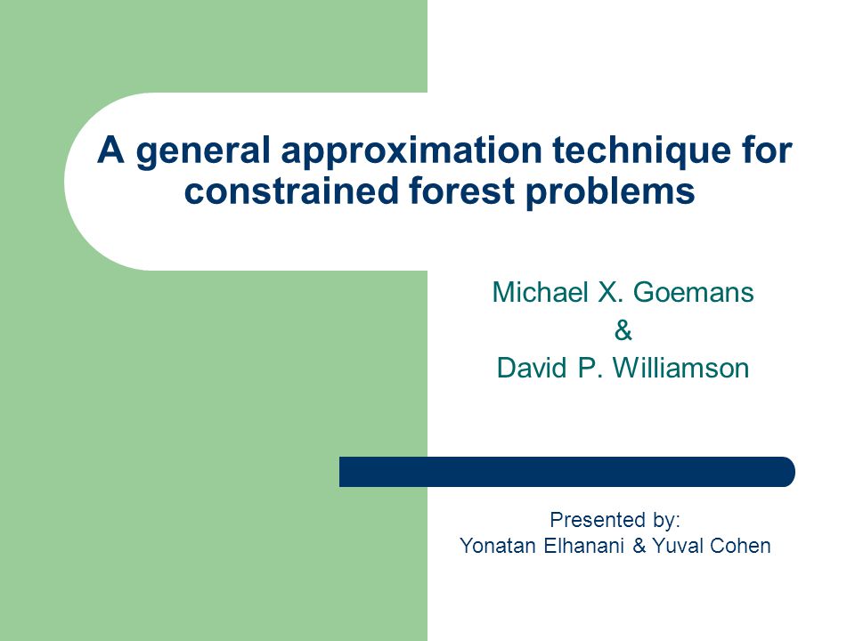
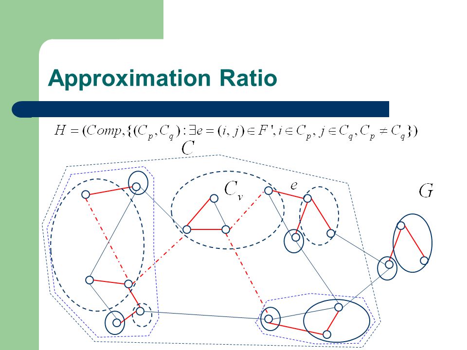
67. Approximation Ratio We will construct the following graph for each iteration:

68. Approximation Ratio We will now show no leaf in H corresponds to an inactive component in G.

69. Approximation Ratio

74. By the construction of, which is a contradiction.

75. Approximation Ratio In the graph, the degree of vertex corresponding to component must be. Let be the set of vertices corresponding to active[inactive] components.

76. Conclusion We proved the algorithm is a -approximation algorithm for the constrained forest problem. We now have a -approximation algorithm for any constrained forest problem.

77. Final Words… The End