1. Dissecting the Milky Way with SDSS: Stellar Number Density Distribution Mario Juric, mjuric@astro.princeton.edu with Z. Ivezic, A. Brooks, R.H.Lupton, D. Schlegel, D. Finkbeiner, N. Padmanabhan, N. Bond, C.M. Rockosi, G.R. Knapp, J.E. Gunn, D.A. Golimowski and the SDSS collaboration July 18 th 2005, LG 2005, Cambridge, UK

2. Mapping the Milky Way structure Top left: SDSS RR Lyrae and other luminous tracers, and 2MASS M giants, demonstrate that the Milky Way halo extends to ~100 kpc and has a lot of substructure What is the structure of the disk component out to a few tens of kpc? SDSS has obtained excellent photometric data for close to 100 million stars. How can one utilize these data for studying the disk component? Bottom left: a schematic representation of the distance range probed by SDSS- detected main sequence stars (out to ~15 kpc)

3. Overview of SDSS Imaging and Spectroscopic Survey ~10,000 deg 2 (1/4 of the full sky) 5 bands (ugriz: UV-IR), 0.02 mag photometric accuracy < 0.1 arcsec astrometric accuracy Over 100,000,000, mostly main sequence, stars Spectra for >200,000 stars (radial v to ~10 km/s) Advantages for studying the Milky Way structure Accurate photometry: photometric distance estimates Numerous stars: small random errors for number density Large area and faint limit: good volume coverage

4. Photometric paralax relation Adopted a single relation that agrees with geometric parallax measurements for nearby M dwarfs, and with globular cluster CMDs. Applied to 48 million stars in 6500 deg 2 and 100 pc to 15 kpc distance range Pitfalls: systematic errors in adopted relation (e.g. metallicity effects), contamination by giants, smaller distance range than for e.g. red giants and RR Lyrae

5. Dissecting the Milky Way with SDSS Traditional approach: assume initial mass function, fold with models for stellar evolution; assume mass-luminosity relation; assume some parametrization for the number density distribution; vary (numerous) free parameters until the observed and model counts agree. Uniqueness? Validity of all assumptions? Our approach: adopt color-luminosity relation, estimate distance to each star, bin the stars in (x,y,z) or (R,Z) space and directly compute the stellar number density (for each narrow color bin). There is no need to a priori assume,the number of, and analytic form for Galactic components

6. - Real 3-D map of the Galaxy - Looking for deviations from axisymmetric models - Better signal-to-noise - Fitting axisymmetric models

7. r - i D [kpc] The r-i color bins sample a variety of scales 15 13 7 4 3 2 1.5 1 0.1 0.2 0.4 0.6 0.8 1 1.2 1.4 SpT ~F9 G6 K4 K7 M0 M1 M2 M3 1 9 r – i c o l o r b i n s – 1 9 d e n s i t y m a p s 0.35 < r-i < 0.40 1.3 < r-i < 1.4

8. (R, Z) density maps 1/5 Notes: - nice exponential structure - very smooth density distribution

9. (R, Z) density maps 2/5 Notes: - distribution still smooth - deviation from simple exponential - addition of thick disk required for acceptable model fits

10. (R, Z) density maps 3/5 Notes: - domination of thick disk - deviations from thin+thick disk models for |Z| > 3kpc

11. (R, Z) density maps 4/5 Notes: - need for an additional component to describe the |Z|>3kpc tails of the distribution - stellar halo

12. (R, Z) density maps 5/5 Notes: - complex density distribution - strong, localized, overdensities

13. Modeling the smooth component Removal of obvious clumps Fit to least “contaminated” bins Exponential disks + halo models Sech 2 models for disks Miyamoto & Nagai (1975) profile

14. Best fit parameters R=8 kpc cross-sections and model predictions

15. The vertical (Z) distribution of SDSS stellar counts for R=8kpc, and 0.1 < r-i < 0.15 color bin. Stars are separated by their u-g color, which is a proxy for metallicity, into a sample representative of the halo stars ( 0.60 < u-g < 0.95 ) and a sample representative of the disk stars ( 0.05 < u-g < 1.15 ). The dashed lines in the bottom two panels are best fit models for the halo and the disk (thick+thin). Stars comprising the halo component are physically different from disk stars. Physicallity of model components

16. Model fit residuals Data Model D/M-1 1.3 < r-i < 1.4 1.1 < r-i < 1.20.8 < r-i < 0.90.35 < r-i < 0.40 Scale increases this way

17. The Milky Way - 2 exponential disks + 1 oblate halo + Numerous clumps, both in the disk and the halo! - Halo “flaring”? - 20-40 clumps expected within the whole disk (have we found the “missing satellites”?)

18. “Virgo overdensity” For high Z, the maximum of our density distribution started shifting away from the Galactic center. We identify this as being caused by a large, localized, overdensity feature in the direction l~300, b~60. Glimpses of this feature were seen in QUEST survey (Vivas et al) and in Newberg et al. 2001.

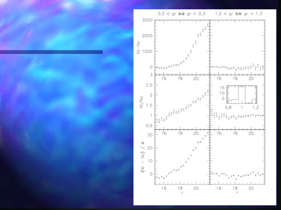
19. Verification of Virgo Overdensity Top left: number density of stars with 0.2 < g-r < 0.3 and 20 < r < 21 in the northern sky shown in Lambert equal- area projection (NGP in the center, GC to the left). Corresponds to a shell in space. Top and bottom right panels: Hess diagrams for two 540deg 2 large regions marked “Virgo” and “Control”. Bottom left panel is the difference. L R

20. Metallicity Stars in the overdensity show metallicity lower than the disk stars, comparable to metallicity of the halo. lower metalicity higher metalicity

21. The Nature of Virgo Overdensity A localized feature Almost perpendicular to the Galactic plane Extends over ~1000deg 2 on the sky Extent: 5kpc < Z < 15kpc, R ~ 8kpc diameter ~ 5kpc Most likely a new tidal stream, possibly a remnant as well? A low metallicity dwarf galaxy progenitor?

22. Summary We have built 19 three-dimensional stellar number density maps of the Milky Way from SDSS photometric observations of stars (~48 million) A two-component exponential disk model, plus an oblate halo give the best fit to the smooth data. Halo power law index and normalization are poorly constrained, due to confusion with clumps and overdensities. However, an oblate halo is always preferred. Clumps/overdensities/streams are an integral part of Milky Way structure, both of halo and the disk(s). We find a remarkably large, localized, overdensity in the direction of constellation Virgo spanning over ~1000deg 2 of the sky We do not find strong evidence for stellar halo triaxiality (Juric et al., in prep.)

25. Studying the deviations from the models in full 3D maps A galactocentric X-Y slice at given Z (height above the Galactic plane) for a given r-i bin. Galactic center is to the left. Dashed circles are circles of constant cylindrical radius around the Galactic center. The number density is color-coded (natural log scale).

26. Also know as the “SDSS ring around the Galaxy”, a tidal stream of stars roughly parallel to the Galactic plane at R~18kpc We see it clearly as a density enhancement at 14kpc < R < 18kpc and 3kpc < Z < 6kpc. Effectively a test of our photometric paralax method. Monoceros overdensity (Newberg et al., 2001)

27.  = 30deg Middle: Crossections through the overdensity (as show on the figure above). Far right: Number density vs. R through the crossection for different heights Z above the plane [top to bottom: (6,7,8), (8,9,10) and (11,12,13) kpc].

28. Later today! Exclusive one-time offer! Two for the price of one! From the same authors who went over time with “Milky Way Tomography with SDSS”!

29. SDSS Photometry

30. Bayesian estimation of stellar colors Stellar locus Prior Likelihood

31. Improving precision, reducing bias

32. Using measured colors Using estimated colors

33. Calculating the surveyed volume Tricky because of Tricky because of complex geometry complex geometry incomplete coverage incomplete coverage overlap of runs overlap of runs We developed an algorithm that can handle arbitrary observing geometry on the sky We developed an algorithm that can handle arbitrary observing geometry on the sky

34. Number density maps 19 r-i bins 19 r-i bins r min =15, r max =21.5 r min =15, r max =21.5 Volume limited Volume limited

35. The bane of pencil-beam surveys: degeneracies To discern between disk+disk and disk+halo models, one needs full (R,z) coverage. We find the halo to be oblate. Thinks to note about modelling I

36. The radial distribution of SDSS stellar counts for different r-i color bins, and at different heights above the plane, as marked on each panel. The two dashed lines show the exponential radial dependence of density for scale lengths of 3000 and 5000pc (with arbitrary normalization). From the available data, it is hard to get a good constraint on the exponential scale length. Thinks to note about modelling III

37. Thinks to note about modelling IV Radial distributions of SDSS stellar counts for 0.1 < r-i < 0.15 color bin The selected heights (Z) are, from top to bottom, (2,3,4), (4,5,6), (6, 8, 10) kpc. Note a significant deviation from exponentiallity, in two overdensities at R~18kpc (Monoceros stream) and R~5kpc (?).

38. Basic concept Fundamental equation: Fundamental equation: Use SDSS imaging observations of stars Use SDSS imaging observations of stars Estimate distances using the photometric paralax method Estimate distances using the photometric paralax method Calculate the volume covered during imaging Calculate the volume covered during imaging Divide Divide

39. SDSS imaging footprint as of DR3+

40. The sample 248 SDSS imaging runs 248 SDSS imaging runs 5457deg 2 north 5457deg 2 north 1081deg 2 south 1081deg 2 south 122 million observations 122 million observations Culled to 73 million after requiring r < 22 m and the existence of g or i magnitude measurements Culled to 73 million after requiring r < 22 m and the existence of g or i magnitude measurements Positionally matched to 47.7 million unique point sources (stars) Positionally matched to 47.7 million unique point sources (stars) 17.2 million stars with multiepoch observations! 17.2 million stars with multiepoch observations! Calculate mean magnitudes, account for extinction Calculate mean magnitudes, account for extinction

41. Can the Virgo overdensity explain recent triaxial halo claims? - Newberg & Yanny (astro-ph/0502386) - The overdensity confuses the interpretation of the star counts - It seems to be a factor significantly responsible for the triaxial halo interpretation - In our 3D maps and model fits we do not find strong evidence for stellar halo triaxiallity