Download presentation
Presentation is loading. Please wait.

1
Dynamics of biological switches 2. Attila Csikász-Nagy King’s College London Randall Division of Cell and Molecular Biophysics Institute for Mathematical and Molecular Biomedicine

2
Dynamical Systems Theory

3
y x dx/dt=f(x,y) dy/dt=g(x,y) (x o,y o ) x=f(x o,y o ) t y=g(x o,y o ) t Phase plane Two variable system: Nullclines = balance curves
 dy/dt=g(x,y) (x o,y o ) x=f(x o,y o ) t y=g(x o,y o ) t Phase plane Two variable system: Nullclines = balance curves")
4
Phase space stable point (node) unstable point (saddle) trajectory Vector field separatrix S S U
 unstable point (saddle) trajectory Vector field separatrix S S U")
5
Unstable – a saddle-point one stable direction, and one unstable direction

6
Phase space stable point (node) unstable point (saddle) trajectory Vector field separatrix S S U
 unstable point (saddle) trajectory Vector field separatrix S S U")
7
Bifurcation: change in number or stability of steady states Saddle-Node bifurcation: one saddle and one node disappear S

8
limit cycle Hopf bifurcation: one node changes stability and a limit cycle is born Bifurcation: change in number or stability of steady states

9
MPF Cyclin Phase Plane dx/dt=f(x,y) dy/dt=g(x,y)
 dy/dt=g(x,y)")
10
MPF Cyclin Phase Plane dx/dt=f(x,y) dy/dt=g(x,y)
 dy/dt=g(x,y)")
11
MPF Cyclin Phase Plane dx/dt=f(x,y) dy/dt=g(x,y)
 dy/dt=g(x,y)")
12
Hopf Bifurcation

13
One-parameter bifurcation diagram parameter variable stable steady state unstable steady state saddle-node Hopf Signal Response t t p x OFF ON (signal) (response) hysteresis bistability oscillation
 (response) hysteresis bistability oscillation")
14
parameter (signal) variable (response) saddle-node Hopf Signal – response curve steady state change – can be visualized for any variable time independent – only steady state matters
 variable (response) saddle-node Hopf Signal – response curve steady state change – can be visualized for any variable time independent – only steady state matters")
15
parameter (signal) variable (response) saddle-node Hopf Second Parameter supercritical
 variable (response) saddle-node Hopf Second Parameter supercritical")
16
parameter (signal) variable (response) Hopf Second Parameter subcritical Second Parameter cyclic fold
 variable (response) Hopf Second Parameter subcritical Second Parameter cyclic fold")
17
parameter (signal) variable (response) Second Parameter SN unstable SNIC or SNIPER
 variable (response) Second Parameter SN unstable SNIC or SNIPER")
18
Two-parameter bifurcation diagram First parameter Second parameter SN Hopf (super) Hopf (sub) SNIC SL BISTABILITY OSCILLATIONS CF 3 3 2 2 1 1
 Hopf (sub) SNIC SL BISTABILITY OSCILLATIONS CF")
19
Molecular Network Dynamics http://www.silva.bsse.ethz.ch/cobi/education/Math_Mod_basic

21
R S response (R) signal (S) linear S=1 5 0 00.51 R rate (dR/dt) rate of degradation S=2 S=3 Gene Expression Signal-Response Curve Bifurcation diagram k1k1 k2k2 rate of synthesis
 signal (S) linear S= R rate (dR/dt) rate of degradation S=2 S=3 Gene Expression Signal-Response Curve Bifurcation diagram k1k1 k2k2 rate of synthesis")
23
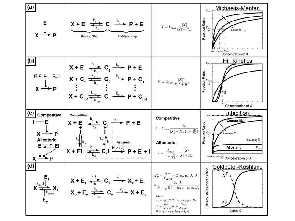
R Kinase RP ATP ADP H2OH2O PiPi Protein Phosphorylation 0.5 1 2 Phosphatase response (RP) Signal (Kinase) “Buzzer” Goldbeter & Koshland, 1981 1.5 0.25 RP 1 R 0 rate (dRP/dt) 1 2 0 00.51
 Signal (Kinase) Buzzer Goldbeter & Koshland, RP 1 R 0 rate (dRP/dt)")
24
Multisite modification

25
Progress in Biophysics and Molecular Biology (2009) 100, 1–3, 47–56
 100, 1–3, 47–56")
26
Multisite modification

27
Switches Buzzer

28
Switches Buzzer

29
Switches Buzzer Toggle switch One way switch

30
Switches Buzzer Toggle switch One way switch Irreversible switch Reversible switch

31
R S EP E R rate (dR/dt) S=0 S=8 S=16 response (R) signal (S) Positive Feedback on synthesis Bistability Griffith, 1968
 S=0 S=8 S=16 response (R) signal (S) Positive Feedback on synthesis Bistability Griffith, 1968")
32
Example: response (R) signal (S) dying Apoptosis (Programmed Cell Death) living
 signal (S) dying Apoptosis (Programmed Cell Death) living")
33
R S EP E R rate (dR/dt) response (R) signal (S) S=0.6 S=1.2 S=1.8 SN Mutual Inhibition on degradation Bistability neg x neg = positive EEP
 response (R) signal (S) S=0.6 S=1.2 S=1.8 SN Mutual Inhibition on degradation Bistability neg x neg = positive EEP")
34
Negative Feedback Loop

35
S X Y YP R RP time X YP RP response (RP) signal (S) Hopf Negative Feedback Loop Goodwin, 1965
 signal (S) Hopf Negative Feedback Loop Goodwin, 1965")
36
R S EP E X X R Positive Feedback & Substrate Depletion positive substrate signal (S) Hopf response (R) “Blinker” Glycolytic Oscillations Oscillation relaxation oscillation sss uss Higgins, 1965; Selkov, 1968
 Hopf response (R) Blinker Glycolytic Oscillations Oscillation relaxation oscillation sss uss Higgins, 1965; Selkov, 1968")
37
Combining positive and negative feedback loops

38
Sources of nonlinearity Oligomer binding Cooperativity and allostery Multisite regulation Stochiometric inhibition

39
R S X R rate (dR/dt) S=1 S=3 S=2 S X R time Sniffer Response is independent of Signal (Levchenko & Iglesias, 2002)
 S=1 S=3 S=2 S X R time Sniffer Response is independent of Signal (Levchenko & Iglesias, 2002)")
41
Example: Bacterial Chemotaxis Barkai & Leibler, 1997 Goldbeter & Segel, 1986 Bray, Bourret & Simon, 1993

42
Two component motifs total: 3 4 = 81 3 2 = 9 (6) Three component motifs total : 3 9 = 19683 3 6 = 729 (138) With inhibitory self interactions:
 Three component motifs total : 3 9 = = 729 (138) With inhibitory self interactions:")
43
Chaotic behavior in a three component network

44
Stochastic models can fit partial viability Tyers, M. (1996). The cyclin-dependent kinase inhibitor p40 SIC1 imposes the requirement for Cln G1 cyclin function at Start. Proc. Natl. Acad. Sci. USA 93:7772- 7776. Nugroho, T.T. and Mendenhall, M.D. (1994). An inhibitor of yeast cyclin-dependent protein kinase plays an important role in ensuring the genomic integrity of daughter cells. Mol. Cell. Biol. 14:3320-3328. Journal of Theoretical Biology (in press: doi:10.1016/j.jtbi.2008.07.019 ) Stochastic Petri Net extension of a yeast cell cycle model Ivan Mura, Attila Csikász-Nagy
. The cyclin-dependent kinase inhibitor p40 SIC1 imposes the requirement for Cln G1 cyclin function at Start. Proc. Natl. Acad. Sci. USA 93: Nugroho, T.T. and Mendenhall, M.D. (1994). An inhibitor of yeast cyclin-dependent protein kinase plays an important role in ensuring the genomic integrity of daughter cells. Mol. Cell. Biol. 14: Journal of Theoretical Biology (in press: doi: /j.jtbi ) Stochastic Petri Net extension of a yeast cell cycle model Ivan Mura, Attila Csikász-Nagy.")
45
time n(t) n is a continuous variable discrete description Time interval between steps: Impossible: system should keep track of time between event occurrences There is no clock in this system – no memory of the past Response depends only on present conditions: MARKOV PROCESS n k
 n is a continuous variable discrete description Time interval between steps: Impossible: system should keep track of time between event occurrences There is no clock in this system – no memory of the past Response depends only on present conditions: MARKOV PROCESS n k ")
46
MARKOV PROCESS Reactions occur with some probability per unit time, proportional to the reaction rates distribution of possible values

47
N small sub time intervals Chance that a reaction occurs in any of these small intervals: rT/N Given that dt = T/N, the chance that a reaction occurs in this small interval is: rdt Define: p n (t) – number of these systems which have n molecules at time t Consider identical systems with the same initial conditions this number can increase if X is created in a system having n-1 molecules, or if X is destroyed in a system having n+1 molecules
 – number of these systems which have n molecules at time t Consider identical systems with the same initial conditions this number can increase if X is created in a system having n-1 molecules, or if X is destroyed in a system having n+1 molecules ")
48
Include all four fluxes: Master equation: Divide the number of systems in a given state n by the fixed number of systems gives p n (t) as the probability for any given system to be in state n example: p n represents the fraction of cells having n copies of some proteins in a population of cells
 as the probability for any given system to be in state n example: p n represents the fraction of cells having n copies of some proteins in a population of cells")
49
we expect deviations from deterministic behavior of the order of the inverse square root of the number of molecules involved average 20 moleculesaverage 500 molecules

50
Suppose a chemical reaction occurs with rate r. What is the time interval between successive occurrences of the reaction? - The probability that the reaction occurs in some time interval dt is rdt - The probability that it does not occur is therefore 1 – rdt The probability that it occurs only after some time can be calculated as follows: Set implies but

51
gives The waiting times between successive reactions are therefore exponentially distributed, with mean value, and variance If u is a random number drawn from a uniform distribution between zero and one, then the following function of u is distributed precisely as is in mm rmrm AmBmAmBm ::: r2r2 A2B2A2B2 r1r1 A1B1A1B1 MIN ( 1, 2, …, m ) = Next steps: Chose reaction Update system Recalculate r and “simplified Gillespie algorithm”
 = Next steps: Chose reaction Update system Recalculate r and simplified Gillespie algorithm")
52
Gillespie method: More reactions: a 0 – sum of all reaction rates Another uniform distribution random number Next step: Update system

53
Lifetime of a state depending on molecule number Again for large molecule number we got back the deterministic solution – stable steady state (Switch rate can determine molecule number)
")
54
Petri nets are a graphical modeling formalism with an intuitive mapping into biochemical transformations A + B → C k A B C k From reactions to Petri nets

55
From continuous to discrete kinetics Mapping concentrations into equivalent number of molecules For each species, proportionality between number of molecules and concentration is given by a scaling constant conversion factor α -1 accounts for 505 molecules per cell = 1 μM Mapping ODE terms into transition rates

56
Translation into a Petri Net The model has been encoded using Möbius

57
Experimental and model results Tyers, M. (1996). The cyclin-dependent kinase inhibitor p40 SIC1 imposes the requirement for Cln G1 cyclin function at Start. Proc. Natl. Acad. Sci. USA 93:7772- 7776.

58
CKI deleted - sic1Δ Experimental results: mutant is viable, but “sick”. Many cells die with mitotic delay. Both models indicate the viability of the mutant –BUT the SPN solution shows many irregularities in the cell cycle, matching the real phenotype Nugroho, T.T. and Mendenhall, M.D. (1994). An inhibitor of yeast cyclin-dependent protein kinase plays an important role in ensuring the genomic integrity of daughter cells. Mol. Cell. Biol. 14:3320-3328.
. An inhibitor of yeast cyclin-dependent protein kinase plays an important role in ensuring the genomic integrity of daughter cells. Mol. Cell. Biol. 14:")
59
Investigation on the mutant with CKI deleted 500 batches of simulation, 95% confidence level Variability of the mutant vs wild type –the results show a significant difference in the spread of both cycle time and mass Experimental results also show high variability of cell cycle times Nugroho, T.T. and Mendenhall, M.D. (1994). Mol. Cell. Biol. 14:3320-3328. Wild Type sic1
. Mol. Cell. Biol. 14: Wild Type sic1 .")
60
Investigation on sic1Δ mutant Wild type sic1 Wild type sic1 Nugroho, T.T. and Mendenhall, M.D. (1994). An inhibitor of yeast cyclin- dependent protein kinase plays an important role in ensuring the genomic integrity of daughter cells. Mol. Cell. Biol. 14:3320-3328.
. An inhibitor of yeast cyclin- dependent protein kinase plays an important role in ensuring the genomic integrity of daughter cells. Mol. Cell. Biol. 14:")
61
Spatial modeling

62
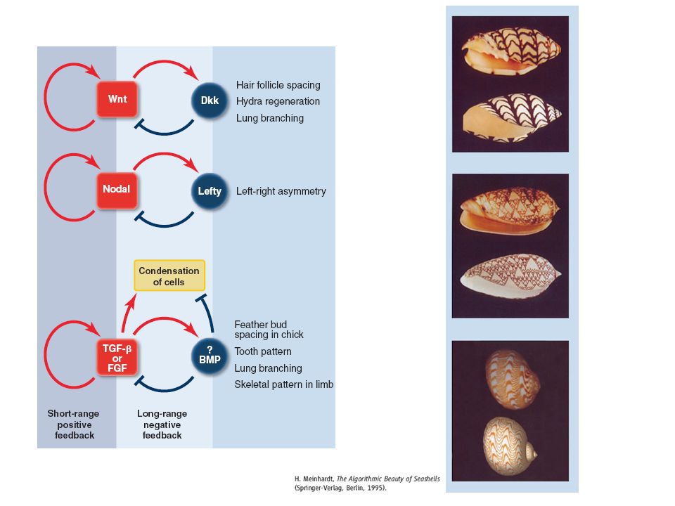
Two different pattern formation mechanisms primary gradient threshold 1 threshold 2 interpretation of gradient establishment of a new gradient positional information self-organized gradient local self-enhancement long range inhibition L. Wolpert (1969) A.M. Turing (1952); A. Gierer & H. Meinhardt (1972)
 A.M. Turing (1952); A. Gierer & H. Meinhardt (1972).")
64
Permanent sensitivity is achieved by generation of local signals and their subsequent local destabilization H. Meinhardt J. Cell Sci. (1999) 112, 2867-2874
 112,")
Similar presentations


 Supervisor: Dr. Rui Alves.>")


 and Elowitz (repressilator) to inform design of biological network necessary to encode.>")

