1. The Time Value of Money Schweser CFA Level 1 Book 1 – Reading #5 master time value of money mechanics and crunch the numbers

2. #5 The time value of money  LOS 5.a - Interest rate interpretation  LOS 5.b - Real risk-free rate and premiums  LOS 5.c - Effective annual rate (EAR)  LOS 5.d - Different frequencies of compounding  LOS 5.e - Present value (PV); future value (FV); annuity  LOS 5.f - Solution by timeline demonstration  Concept checkers

3. Time Lines  Draw time lines to better show the cash flows  Cash Inflow: positive; you receive money  Cash Outflow: negative; you pay money  Present value (PV): discount all future cash flows into today’s value  Future value (FV): compound all cash flows to the value of a future date  N = Number of compounding periods  I/Y = Interest rate of compounding periods  PMT = Payment, periodic cash flow  CPT = compute

4. Time Lines  Time Line demonstration.  T = 0, today, cash outflow = 1000  Time length : 8 years  At the end of each year : cash inflow = 600  Blue numeric numbers from 1 to 8: end of 1 st year … end of 8 th year  End of 1 st year = beginning of 2 nd year  End of year i = beginning of year i+1 -1000 +600 0 1 2 3 4 5 6 7 8

5. LOS 5.a Interpret interest rates as required rates of return, discount rates, or opportunity costs

6.  Compound Interest or Interest on Interest: the interest earned on the previous period's interest earnings.  Interest rate interpretation  Required rate of return: the required return at which investors will invest  Discount rates: borrow rate of investors from banks, as he will pay the interest  Opportunity cost of current consumption: This is value of the best alternative foregone, or in other words, this is the return of something else that you have to give up when consume in this project.

7. LOS 5.b Explain an interest rate as the sum of a real risk-free rate, and premiums that compensate investors for bearing distinct types of risk

8.  Risk free rate: The interest rate without any potential risks  Nominal risk-free rate = real risk-free rate + expected inflation rate (e.g., U.S. Treasury bill (T-bills) )  Real risk-free rate: has no expectation of inflation in itinvestor’s increase in purchasing power (after adjusting for inflation)  Types of risks (risks of securities contain the first three types of risks):  Default risk: ex. Firms unable to pay back its debt (bonds)  Liquidity risk: ex. Sell securities for cash less than fair value in illiquid markets  Maturity risk: ex. Long term bonds are more volatile  Exchange rate risk: change in exchange rate if you buy or sell in foreign currency.  ….  Required interest rate: the sum of nominal risk-free rate and risk premiums  Nominal risk-free rate +  Default risk premium +  Liquidity premium +  Maturity risk premium…  (premium: additional part as compensation for additional risk)

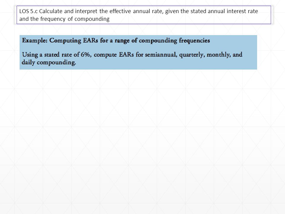
9. LOS 5.c Calculate and interpret the effective annual rate, given the stated annual interest rate and the frequency of compounding

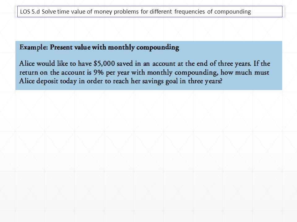
15. LOS 5.d Solve time value of money problems for different frequencies of compounding We need to consider the case of compounding periods are other than annual, or the frequencies of compounding are different than annual.

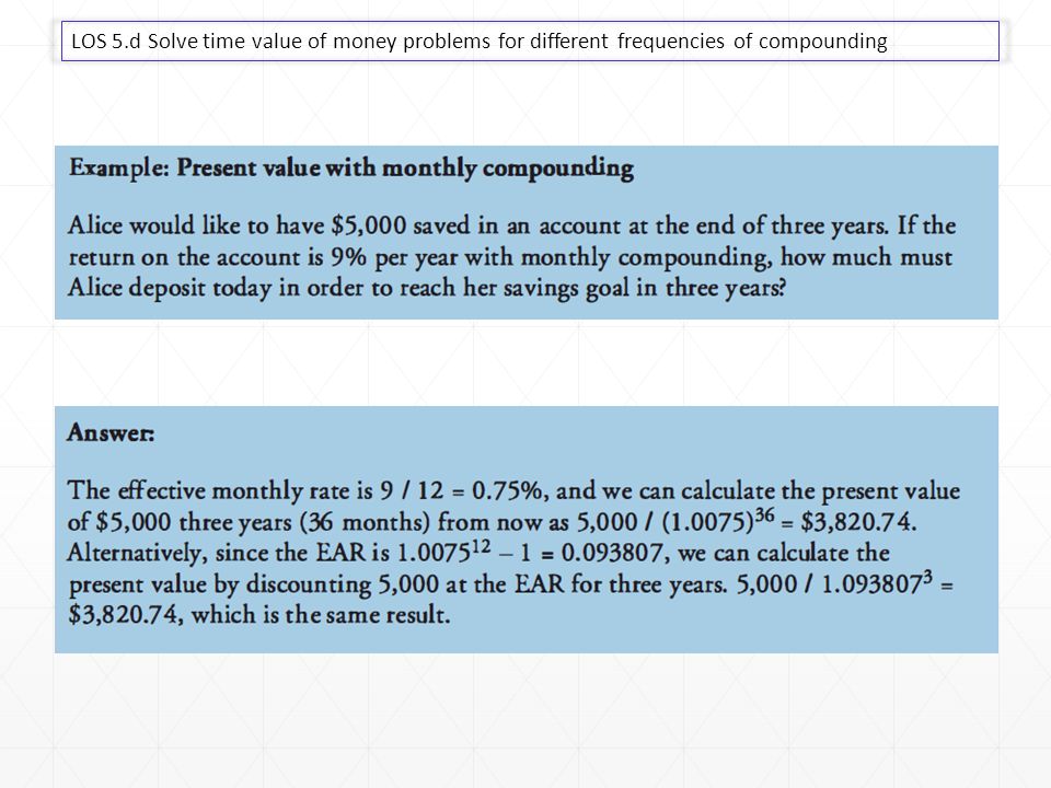
16. LOS 5.d Solve time value of money problems for different frequencies of compounding

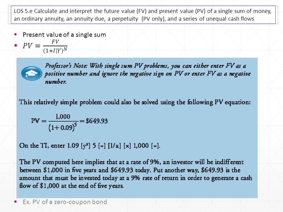
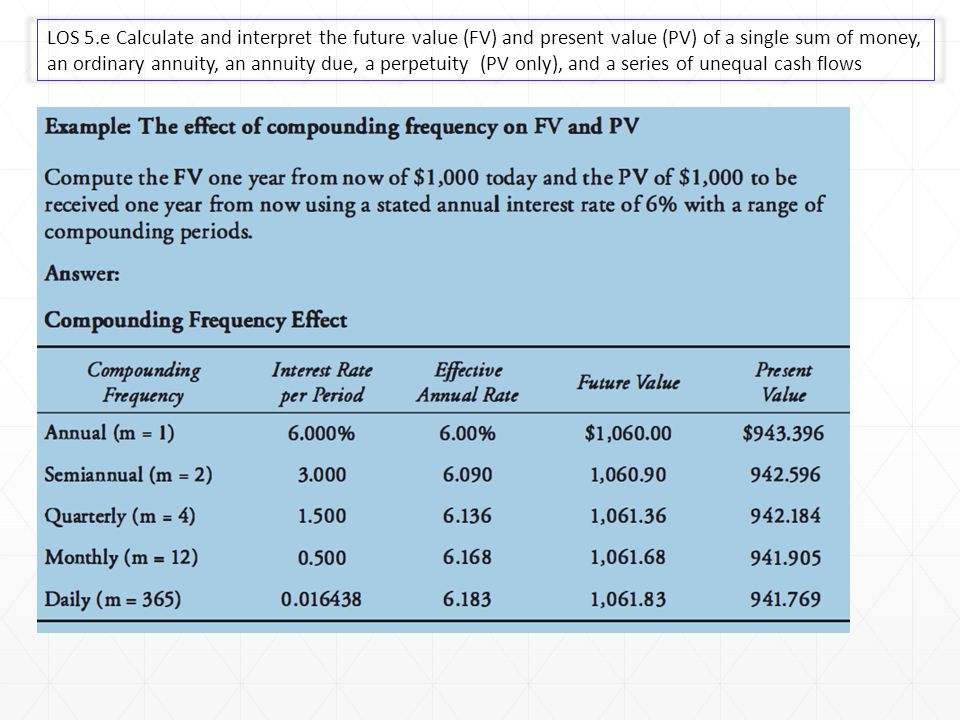
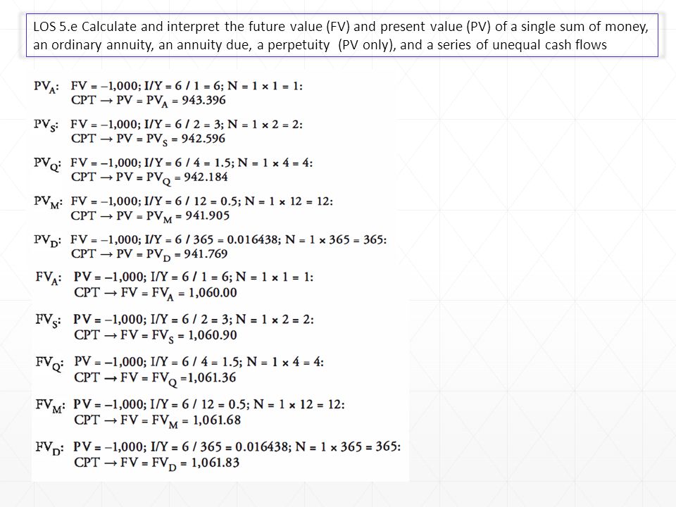
19. LOS 5.e Calculate and interpret the future value (FV) and present value (PV) of a single sum of money, an ordinary annuity, an annuity due, a perpetuity (PV only), and a series of unequal cash flows

25.  Annuities: An annuity is a series of equal dollar payments that are made at the end of equidistant points in time such as monthly, quarterly, or annually over a finite period of time.  Ex. Receiving $1000 per year at the end of next 8 years  Ordinary annuities: If payments are made at the end of each period, the annuity is referred to as ordinary annuity.

26. LOS 5.e Calculate and interpret the future value (FV) and present value (PV) of a single sum of money, an ordinary annuity, an annuity due, a perpetuity (PV only), and a series of unequal cash flows  You can use the following formula to calculate FV of an ordinary Annuity

27. LOS 5.e Calculate and interpret the future value (FV) and present value (PV) of a single sum of money, an ordinary annuity, an annuity due, a perpetuity (PV only), and a series of unequal cash flows  You can use the formula in previous slide or use calculator to crunch the result as follows:

28. LOS 5.e Calculate and interpret the future value (FV) and present value (PV) of a single sum of money, an ordinary annuity, an annuity due, a perpetuity (PV only), and a series of unequal cash flows  Mathematic formula to calculate the Present value of

29. LOS 5.e Calculate and interpret the future value (FV) and present value (PV) of a single sum of money, an ordinary annuity, an annuity due, a perpetuity (PV only), and a series of unequal cash flows

33. Annuity Due: is an annuity in which all the cash flows occur at the beginning of the period. For example, rent payments on apartments are typically annuity due as rent is paid at the beginning of the month. Computation of future/present value of an annuity due requires compounding the cash flows for one additional period, beyond an ordinary annuity.

34. LOS 5.e Calculate and interpret the future value (FV) and present value (PV) of a single sum of money, an ordinary annuity, an annuity due, a perpetuity (PV only), and a series of unequal cash flows 0 1 2 3 +100 +100 +100 FVA(D) +100 +100 +100 FVA(O)

35. LOS 5.e Calculate and interpret the future value (FV) and present value (PV) of a single sum of money, an ordinary annuity, an annuity due, a perpetuity (PV only), and a series of unequal cash flows

37. 0 1 2 3 +100 +100 +100 PVA(D) +100 +100 +100 PVA(O)

38. LOS 5.e Calculate and interpret the future value (FV) and present value (PV) of a single sum of money, an ordinary annuity, an annuity due, a perpetuity (PV only), and a series of unequal cash flows

40.  Similarly, we can set N as large as possible to get this $56.25  N= 9999; I|Y = 8; PMT = 4.5; FV = 0; [CPT]  [PV] = -56.25

41. LOS 5.e Calculate and interpret the future value (FV) and present value (PV) of a single sum of money, an ordinary annuity, an annuity due, a perpetuity (PV only), and a series of unequal cash flows

42. 0 +4000 +3500 +2000 -1000 -500 0 1 2 3 4 5 6

43. LOS 5.e Calculate and interpret the future value (FV) and present value (PV) of a single sum of money, an ordinary annuity, an annuity due, a perpetuity (PV only), and a series of unequal cash flows

49. LOS 5.f Demonstrate the use of a time line in modeling and solving time value of money problems Loan Amortization Amortized loan: a special type of loan that is paid off by making a series of regular & equal payments Part of each payment goes towards paying off the simple interest from the unpaid balance while the rest goes towards paying off the principal of the loan This differs from installment loans where the interest over the lifetime of the loan is computed at purchase Interest for an amortized loan is computed on the unpaid balance The amount of loan and interest payment do not remain fixed over the term of loan. Examples: House Mortgaged Loans, Auto Loans In an amortized loan, the present value can be thought of as the amount borrowed, n is the number of periods the loan lasts for, i is the interest rate per period, and payment is the loan payment that is made.

50. LOS 5.f Demonstrate the use of a time line in modeling and solving time value of money problems Loan Amortization Interest Component = Beginning Balance * Periodic Interest Rate Principal Component = Payment - Interest Sum of Principal Repayments = Original Amount of Loan Sum of Interest Payments = Sum of Total Payments – Sum of Principal Repayments

51. LOS 5.f Demonstrate the use of a time line in modeling and solving time value of money problems Loan Amortization For Example: Beginning balance of a loan is $100000, interest rate is 10% and loan term is 10 years. What is the installment payment? Construct amortization schedule. Amortization Schedule:

52. LOS 5.f Demonstrate the use of a time line in modeling and solving time value of money problems Loan Amortization For Example: Beginning balance of a loan is $100000, interest rate is 10% and loan term is 10 years. Amortization Schedule:

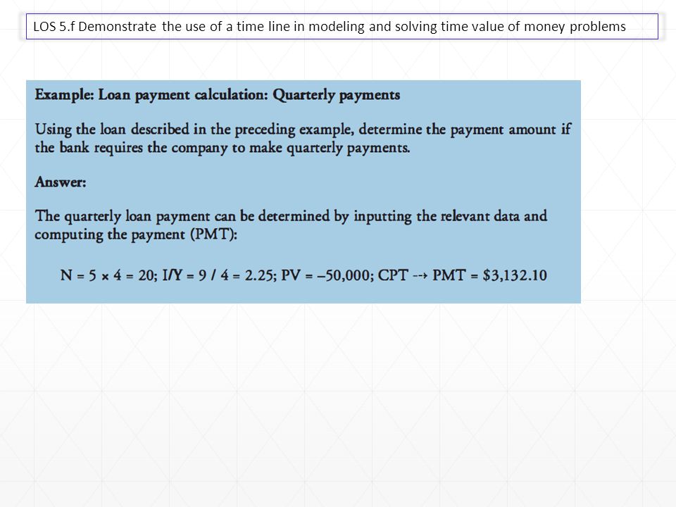
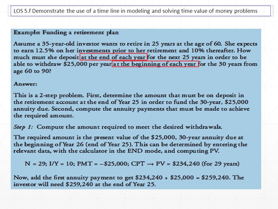
53. LOS 5.f Demonstrate the use of a time line in modeling and solving time value of money problems

56. Note: Once you have solved for the payment, $2637.97, the remaining principal on any payment date can be calculated by entering N = number of remaining payments and solving for the PV For example: N=4, PMT = 2637.97, I|Y = 10, FV = 0, [CPT] -> PV = 8362.03 Note: Once you have solved for the payment, $2637.97, the remaining principal on any payment date can be calculated by entering N = number of remaining payments and solving for the PV For example: N=4, PMT = 2637.97, I|Y = 10, FV = 0, [CPT] -> PV = 8362.03

57. LOS 5.f Demonstrate the use of a time line in modeling and solving time value of money problems Faster method PMT = 802.43 N = 18 I|Y = 5 FV = 0 [CPT] -> PV = 9380.02

58. LOS 5.f Demonstrate the use of a time line in modeling and solving time value of money problems Solving for payment:

59. LOS 5.f Demonstrate the use of a time line in modeling and solving time value of money problems Solving for number of periods:

60. LOS 5.f Demonstrate the use of a time line in modeling and solving time value of money problems

61. Solving for rate of return/discount rate:

62. LOS 5.f Demonstrate the use of a time line in modeling and solving time value of money problems Geometric Mean: The formula for computation of geometric mean in constant time is:

63. LOS 5.f Demonstrate the use of a time line in modeling and solving time value of money problems Putting it all together: Ralph and Alice plan to send their son to a military academy for four years from today. One year’s tuition costs $5,000 today and will increase by 4% per year. How much will they need to invest each year for 5 years, starting today, if they earn 9% on their investments?

64. LOS 5.f Demonstrate the use of a time line in modeling and solving time value of money problems

68. Solving for missing annuity payments: Jim needs $800,000 to retire in 15 years. He will save $20,000 at the end of each of the next five years, and $40,000 at the end of years 11-15. If his investment account returns 11% per year, what equal payments must he make into the account at the end of years 6 thru 10?

69. LOS 5.f Demonstrate the use of a time line in modeling and solving time value of money problems The connection Between PV, FV and Series of Cash Flows Alternative interpretation of present value: How much money you put in the bank today In order to make future withdraws The final withdraw will exhaust the account PV of 100, 200, 300 for the following 3 years will be 481.5928, the assumed interest rate is 10%. This is similar to invest 481.5928 now, and withdraw 100, 200, 300 for each year of the following 3 years, the money in account will generate interest but finally just be offset by the final with draw of 300 Another way is to look at future values of this 3 cash flows for 641 PVCF 0123 100200300 Comp ratio1.11.211.331 PV90.90909165.2893225.3944 Sum(PV)481.5928 CF1CF2CF3 Invest481.5928529.7521472.7273300 Withdraw100200300 Balance429.7521272.72730

70. LOS 5.f Demonstrate the use of a time line in modeling and solving time value of money problems Cash Flow additivity principle: It refers to the present value of any stream of cash flows equal the sum of the present values of the cash flows. The sum of the two series of cash flows is same as the present values of the two series taken together. Example: If we have 3 projects 1 2 and 3, each project’s cash flows are indicated in the table below We compute the PV, and what do we observe? Indeed, the P3 CF = P1 CF + P2 CF if we add each period Project 1 and Project 2 cash flows, we get Project 3 The PV show the same result that PV3 = PV1 + PV2 = 316.9865 + 225.3944 = 542.381 This is a demonstration of the additivity principle rate = 10%1234PV Project 1100 316.9865 Project 2003000225.3944 Project 3100 400100542.381

71. End of Chapter