1. Stephen Alstrup (U. Copenhagen) Esben Bistrup Halvorsen (U. Copenhagen) Holger Petersen (-) Aussois – ANR DISPLEXITY - March 2015 Cyril Gavoille (LaBRI, U. Bordeaux)

2. 1. The Problem 2. Squashed Cube Dimension 3. Dominating Set Technique 4. Another Solution 5. Conclusion Agenda

3. The Distance Labeling Problem Given a graph, find a labeling of its nodes such that the distance between any two nodes can be computed by inspecting only their labels. Subject to: label the nodes of every graph of a family (scheme), label the nodes of every graph of a family (scheme), using short labels (size measured in bits), and using short labels (size measured in bits), and with a fast distance decoder (algorithm) with a fast distance decoder (algorithm) 0000 1111 0001 0011 0111

4. Motivation [Peleg ’99] If a short label (say of poly-logarithmic size) can be added to the address of the destination, then routing to any destination can be done without routing tables and with a “limited” number of messages. dist (x,y) x message header=hop-county

5. A Distributed Data Structure Get the labels of nodes involved in the query Get the labels of nodes involved in the query Compute/decode the answer from the labels Compute/decode the answer from the labels No other source of information is required No other source of information is required

6. Label Size: a trivial upper bound There is a labeling scheme using labels of O(nlogn) bits for every (unweighted) graph G with n nodes, and constant time decoding. L G (i)=(i, [dist(i,1),…,dist(i,j),…,dist(i,n)] ) ➟ distance vector

7. Label Size: a trivial lower bound No labeling scheme can guarantee labels of less than 0.5n bits for all n-node graphs (whatever the distance decoder complexity is) Proof. The sequence L G (1),…,L G (n) and the decoder δ(.,.) is a representation of G on n. k+O(1) bits if each label has size k: i adjacent to j iff δ(L G (i),L G (j))=1. n. k + O(1) ≥ log 2 (#graphs(n))=n. (n-1)/2

8. Squashed Cube Dimension [Graham,Pollack ’71] Labeling: word over {0,1,*} Decoder: Hamming distance (where *=don’t care) (where *=don’t care) (graphs must be connected) SC dim (G)≥max{n +,n - } n +/- =#positive/negative eigen- values of the distance matrix of G SC dim (K n )=n-1

9. Squashed Cube Dimension [Winkler ’83] Theorem. Every connected n-node graph has squashed cube dimension at most n-1. Therefore, for the family of all connected n-node graphs: Label size: O(n) bits, in fact nlog 2 3 ~ 1.58n bits Decoding time: O(n/logn) in the RAM model Rem: all graphs = connected graphs + O(logn) bits

10. Dominating Set Technique [G.,Peleg,Pérennès,Raz ’01] Definition. A k-dominating set for G is a set S such that, for every node x ∈ G, dist(x,S) ≤ k. Fact: Every n-node connected graph has a k- dominating set of size at most n/(k+1). Target: Label size: O(n) bits Label size: O(n) bits Decoding time: O(loglogn) Decoding time: O(loglogn)

11. Part 1 dom S (x) = dominator of x, its closest node in S Observation 1: dist(x,y)=dist(dom S (x),dom S (y))+e(x,y) where e(x,y) ∈ [-2k,+2k] Observation 2: One can encode e(x,y) with log 2 (4k+1) bits

12. Part 2 Idea: take a collection of k i -dominating set S i, i=0…t (may intersect) where k 0 =0, |S i |=n/(k i +1), and |S t |=o(n/logn). Denote x 0 =x and x i =dom Si (x i-1 ). Decoder: dist(x,y)=∑ 1≤i≤t e i (x i-1,y i-1 ) + dist(x t,y t ) Time: O(t)

13. Part 3 Decoder: dist(x,y)=∑ 1≤i≤t e i (x i-1,y i-1 ) + dist(x t,y t ) Label size: ∑ 1≤i≤t |S i-1 |. log 2 (4k i +1) + |S t |. O(logn) bits size ≤ n. ∑ 1≤i≤t log 2 (4k i +1)/(k i-1 +1) + o(n) size ≤ n. ∑ 1≤i≤t log 2 (4k i +1)/(k i-1 +1) + o(n) Choose: k i =4 i -1 and t=loglogn ➟ k 0 =0, log 2 (4k i +1)=2i+2, and |S t |=o(n/logn) ➟ size ≤ n. ∑ i≥1 (2i+2)/4 i-1 = n. (56/9) ~ 6.22n bits ➟ time O(t) = O(loglogn) [ k 0…4 =(0,2,15,145,940), k i =exp(k i-1 ), t=log * n, size ~ 5.90n ]

14. Another Solution Label size: n(log 2 3)/2 ~ 0.793n bits Decoding time: O(1)

15. Warm-up (ignoring decoding time) Assume G has a Hamiltonian cycle x 0,x 1,…,x n-1. ➟ dist(x 0,x i ) = dist(x 0,x i-1 ) + e 0 (x i,x i-1 ) where e 0 (x i,x i-1 ) ∈ {-1,0,+1} ➟ dist(x 0,x i ) = ∑ 1≤j≤i e 0 (x j,x j-1 ) Label: L G (x i )=(i, [e i (x i+1,x i ),e i (x i+2,x i+1 ), …]) Size: n(log 2 3)/2 bits by storing only half e i ()’s

16. Applications Assume G is 2-connected. By Fleischner’s Theorem [1974], G 2 has a Hamiltonian cycle x 0,x 1,…,x n-1. So, e 0 (x i,x i-1 )=dist(x 0,x i )-dist(x 0,x i- 1 ) ∈ {-2,-1,0,1,2}. Label size: n(log 2 5)/2 ~ 1.16n bits For every tree T, T 3 is Hamiltonian. So, if G is connected, then G 3 is Hamiltonian and has a labeling scheme with n(log 2 7)/2 ~ 1.41n bits.

17. Constant Time Solution T = any rooted spanning tree of G e x (u) = dist(x,u)-dist(x,parent(u)) ∈ {-1,0,+1} Telescopic sum: if z ancestor of y, then dist(x,y)=dist(x,z)+∑ u ∈ T[y,z) e x (u)

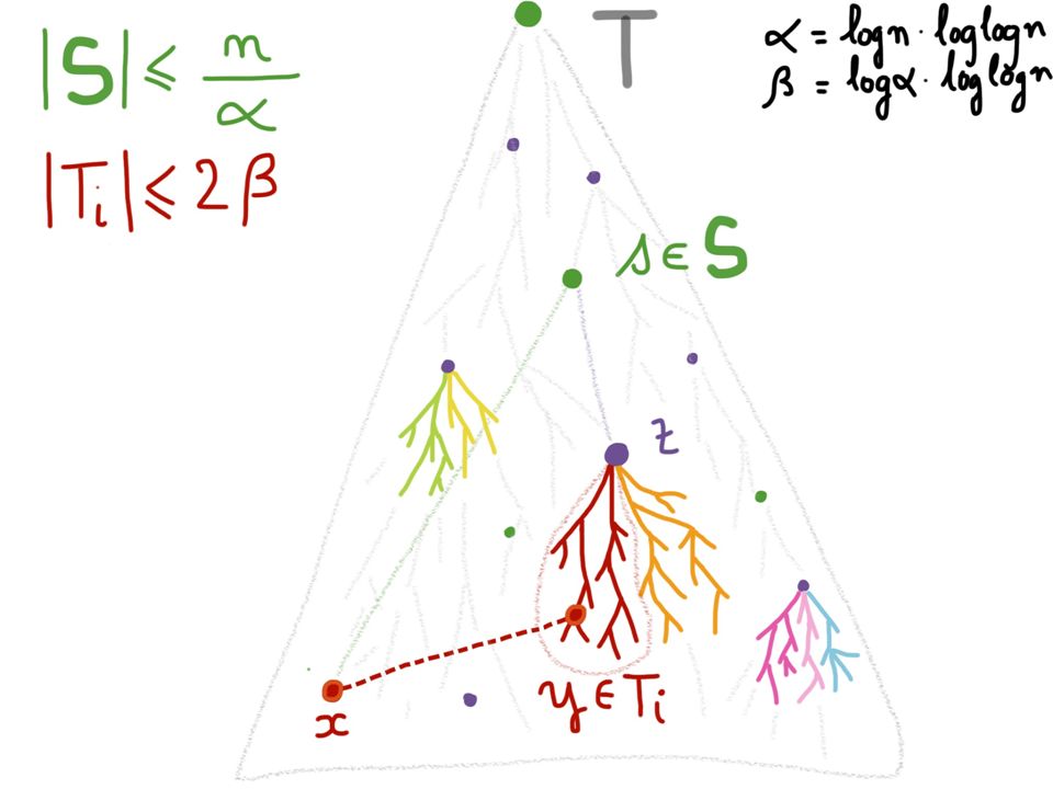
18. Dominating Set & Edge- Partition Select an α-dominating S={s i } with root(T) ∈ S and |S| ≤ (n/α)+1 Edge-partition: T has an edge-partition into at most n/β sub-trees {T i } of ≤ 2β edges. Choose: α=logn. loglogn α=logn. loglogn β=logα. loglogn ~ (loglogn) 2 β=logα. loglogn ~ (loglogn) 2

20. Distance decoder: dist(x,y)=dist(x,z)+∑ u ∈ T[y,z) e x (u) = A + B Storage for computing A: #z logn=(n/β). logn=ω(n) ✖ #z x logn=(n/β). logn=ω(n) ✖ But, A = dist(x,s) + A’, where A’=(dist(x,z)-dist(x,s)) ∈ [-2α,+2α] ➟ only log 2 (2α+1) bits to store A’. #s logn =(n/α). logn = o(n) ✔ #s x logn =(n/α). logn = o(n) ✔ #z log(2α+1)=(n/β). logα = o(n) ✔ #z x log(2α+1)=(n/β). logα = o(n) ✔

21. Distance decoder: dist(x,y)=dist(x,z)+∑ u ∈ T[y,z) e x (u) = A + B Storage for computing B: assume y ∈ T i B=f(T i,e x (T i ),rk(y)) for some f(…) where e x (T i )=[-1,0,+1,+1,0,-1,…] But, the input T i,e x (T i ),rk(y) writes on O(β)=O(log 2 logn) bits! ➟ one can tabulate f(…) once for all its possible inputs with 2 O(β) log 2 B = o(n) bits to have constant time. ➟ one can tabulate f(…) once for all its possible inputs with 2 O(β) x log 2 B = o(n) bits to have constant time. → → →

22. Storage for u (in its label): storage for all A,A’,B ➟ o(n) bits storage also for: 1. i st. u ∈ T i, rk(u) in T i, and z=root(T i ) 2. closest s ∈ S ancestor of z 3. coding of T i with O(β) bits 4. e u (T i ),e u (T i+1 ),… for half the total information (this latter costs n(log 2 3)/2 + o(n) bits) (this latter costs n(log 2 3)/2 + o(n) bits) Decoder: [ x “knows” y, otherwise swap x,y ] 1. y tells to x: i,T i,rk(y),z,s 2. x computes and returns A+A’+B →→

23. Conclusion Main question: Design a labeling scheme with 0.5n+o(n)-bit labels and constant time decoder? Bonus: The technique extends to weighted graphs. We show n. log 2 (2w+1)/2 bits for edge-weight in [1,w]. We show a lower bound of n. log 2 (w/2+1)/2. The technique extends to weighted graphs. We show n. log 2 (2w+1)/2 bits for edge-weight in [1,w]. We show a lower bound of n. log 2 (w/2+1)/2. We also show a 1-additive (one sided error) labeling scheme of n/2 bits, and a lower bound of n/4. We also show a 1-additive (one sided error) labeling scheme of n/2 bits, and a lower bound of n/4.