1. Oded Regev Tel-Aviv University On Lattices, Learning with Errors, Learning with Errors, Random Linear Codes, Random Linear Codes, and Cryptography and Cryptography

2. Outline Introduction to lattices Introduction to lattices Main theorem: a hard learning problem Main theorem: a hard learning problem Application: a stronger and more efficient public key cryptosystem Application: a stronger and more efficient public key cryptosystem Proof of main theorem Proof of main theorem Overview Overview Part I: Quantum Part I: Quantum Part II: Classical Part II: Classical

3. Basis: v 1, …,v n vectors in R n v 1, …,v n vectors in R n The lattice L is L={a 1 v 1 + … +a n v n | a i integers} L={a 1 v 1 + … +a n v n | a i integers} The dual lattice of L is L * ={x | 8 y 2 L, h x,y i 2 Z} Lattices v1v1 v2v2 0 2v 1 v 1 +v 2 2v 2 2v 2 -v 1 2v 2 -2v 1

4. SVP: Given a lattice, find an approximately shortest vector SVP: Given a lattice, find an approximately shortest vector Shortest Vector Problem (SVP) 0 v2v2 v1v1

5. CVP d : Given a lattice and a target vector within distance d, find the closest lattice point CVP d : Given a lattice and a target vector within distance d, find the closest lattice point Closest Vector Problem (CVP d ) 0v

6. Main Theorem Hardness of Learning

7. Learning from parity with error Let s2Z 2 n be a secret Let s2Z 2 n be a secret We have random equations modulo 2 with error (everything independent): We have random equations modulo 2 with error (everything independent): Without error, it’s easy! Without error, it’s easy! s 2 +s 3 +s 4 + s 6 +…+s n  0 s 2 +s 3 +s 4 + s 6 +…+s n  0 s 1 +s 2 + s 4 + s 6 +…+s n  1 s 1 + s 3 +s 4 +s 5 + …+s n  1 s 2 +s 3 +s 4 + s 6 +…+s n  0 s 2 +s 3 +s 4 + s 6 +…+s n  0...

8. More formally, we need to learn s from samples of the form (t,st+e) where t is chosen uniformly from Z 2 n and e is a bit that is 1 with probability 10%. More formally, we need to learn s from samples of the form (t,st+e) where t is chosen uniformly from Z 2 n and e is a bit that is 1 with probability 10%. Easy algorithms need 2 O(n) equations/time Easy algorithms need 2 O(n) equations/time Best algorithm needs 2 O(n/logn) equations/time [ BlumKalaiWasserman’00 ] Best algorithm needs 2 O(n/logn) equations/time [ BlumKalaiWasserman’00 ] Open question: why is this problem so hard? Open question: why is this problem so hard? Learning from parity with error

9. Learning modulo p Fix some p<poly(n) Fix some p<poly(n) Let s2Z p n be a secret Let s2Z p n be a secret We have random equations modulo p with error: We have random equations modulo p with error: 2s 1 +0s 2 +2s 3 +1s 4 +2s 5 +4s 6 +…+4s n  2 0s 1 +1s 2 +5s 3 +0s 4 +6s 5 +6s 6 +…+2s n  4 6s 1 +5s 2 +2s 3 +0s 4 +5s 5 +2s 6 +…+0s n  2 6s 1 +4s 2 +4s 3 +4s 4 +3s 5 +3s 6 +…+1s n  5...

10. Learning modulo p More formally, we need to learn s from samples of the form (t,st+e) where t is chosen uniformly from Z p n and e is chosen from Z p More formally, we need to learn s from samples of the form (t,st+e) where t is chosen uniformly from Z p n and e is chosen from Z p Easy algorithms need 2 O(nlogn) equations/time Easy algorithms need 2 O(nlogn) equations/time Best algorithm needs 2 O(n) equations/time [ BlumKalaiWasserman’00 ] Best algorithm needs 2 O(n) equations/time [ BlumKalaiWasserman’00 ]

11. Main Theorem Learning modulo p is as hard as worst-case lattice problems using a quantum reduction Learning modulo p is as hard as worst-case lattice problems using a quantum reduction In other words: solving the problem implies an efficient quantum algorithm for lattices In other words: solving the problem implies an efficient quantum algorithm for lattices

12. Equivalent formulation For m=poly(n), let C be a random m £ n matrix with elements in Z p. Given Cs+e for some s  Z p n and some noise vector e  Z p m, recover s. For m=poly(n), let C be a random m £ n matrix with elements in Z p. Given Cs+e for some s  Z p n and some noise vector e  Z p m, recover s. This is the problem of decoding from a random linear code This is the problem of decoding from a random linear code

13. Why Quantum? As part of the reduction, we need to perform a certain algorithmic task on lattices As part of the reduction, we need to perform a certain algorithmic task on lattices We do not know how to do it classically, only quantumly! We do not know how to do it classically, only quantumly!

14. Why Quantum? We are given an oracle that solves CVP d for some small d We are given an oracle that solves CVP d for some small d As far as I can see, the only way to generate inputs to this oracle is: As far as I can see, the only way to generate inputs to this oracle is: Somehow choose x  L Somehow choose x  L Let y be some random vector within dist d of x Let y be some random vector within dist d of x Call the oracle with y Call the oracle with y The answer is x. But we already know the answer !! The answer is x. But we already know the answer !! Quantumly, being able to compute x from y is very useful: it allows us to transform the state |y,x> to the state |y,0> reversibly (and then we can apply the quantum Fourier transform) Quantumly, being able to compute x from y is very useful: it allows us to transform the state |y,x> to the state |y,0> reversibly (and then we can apply the quantum Fourier transform) x y

15. Application: New Public Key Encryption Scheme

16. Previous lattice-based PKES [AjtaiDwork96,GoldreichGoldwasserHalevi97,R’03] Main advantages: Main advantages: Based on a lattice problem Based on a lattice problem Worst-case hardness Worst-case hardness Main disadvantages: Main disadvantages: Based only on unique-SVP Based only on unique-SVP Impractical (think of n as  100): Impractical (think of n as  100): Public key size O(n 4 ) Public key size O(n 4 ) Encryption expands by O(n 2 ) Encryption expands by O(n 2 )

17. Ajtai ’ s recent PKES [Ajtai05] Main advantages: Main advantages: Practical (think of n as  100): Practical (think of n as  100): Public key size O(n) Public key size O(n) Encryption expands by O(n) Encryption expands by O(n) Main disadvantages: Main disadvantages: Not based on lattice problem Not based on lattice problem No worst-case hardness No worst-case hardness

18. New lattice-based PKES [This work] Main advantages: Main advantages: Worst-case hardness Worst-case hardness Based on the main lattice problems (SVP, SIVP) Based on the main lattice problems (SVP, SIVP) Practical (think of n as  100): Practical (think of n as  100): Public key size O(n) Public key size O(n) Encryption expands by O(n) Encryption expands by O(n) Breaking the cryptosystem implies an efficient quantum algorithm for lattices Breaking the cryptosystem implies an efficient quantum algorithm for lattices In fact, security is based on the learning problem (no quantum needed here) In fact, security is based on the learning problem (no quantum needed here)quantum

19. The Cryptosystem Everything modulo 4 Everything modulo 4 Private key: 4 random numbers Private key: 4 random numbers 1 2 0 3 Public key: a 6x4 matrix and approximate inner product Public key: a 6x4 matrix and approximate inner product Encrypt the bit 0: Encrypt the bit 0: Encrypt the bit 1: Encrypt the bit 1: 2·1 + 0·2 + 1·0 + 2·3 ≈ 1 1·1 + 2·2 + 2·0 + 3·3 ≈ 2 0·1 + 2·2 + 0·0 + 3·3 ≈ 1 1·1 + 2·2 + 0·0 + 2·3 ≈ 0 0·1 + 3·2 + 1·0 + 3·3 ≈ 3 3·1 + 3·2 + 0·0 + 2·3 ≈ 2 2 0 1 2 1 2 2 3 0 2 0 3 1 2 0 2 0 3 1 3 3 3 0 2 2·? + 0·? + 1·? + 2·? ≈ 1 1·? + 2·? + 2·? + 3·? ≈ 2 0·? + 2·? + 0·? + 3·? ≈ 1 1·? + 2·? + 0·? + 2·? ≈ 0 0·? + 3·? + 1·? + 3·? ≈ 3 3·? + 3·? + 0·? + 2·? ≈ 2 3·? + 2·? + 1·? + 0·? ≈ 3 2·1 + 0·2 + 1·0 + 2·3 = 0 1·1 + 2·2 + 2·0 + 3·3 = 2 0·1 + 2·2 + 0·0 + 3·3 = 1 1·1 + 2·2 + 0·0 + 2·3 = 3 0·1 + 3·2 + 1·0 + 3·3 = 3 3·1 + 3·2 + 0·0 + 2·3 = 3 3·? + 2·? + 1·? + 0·? ≈ 1

20. Proof of the Main Theorem Overview

21. Gaussian Distribution Define a Gaussian distribution on a lattice (normalization omitted) Define a Gaussian distribution on a lattice (normalization omitted) We can efficiently sample from D r for large r=2 n We can efficiently sample from D r for large r=2 n

22. The Reduction Assume the existence of an algorithm for the learning modulo p problem for p=2√n Assume the existence of an algorithm for the learning modulo p problem for p=2√n Our lattice algorithm: Our lattice algorithm: r=2 n r=2 n Take poly(n) samples from D r Take poly(n) samples from D r Repeat: Repeat: Given poly(n) samples from D r compute poly(n) samples from D r/2 Given poly(n) samples from D r compute poly(n) samples from D r/2 Set r←r/2 Set r←r/2 When r is small, output a short vector When r is small, output a short vector

23. DrDr

24. D r/2

25. Obtaining D r/2 from D r Lemma 1: Lemma 1: Given poly(n) samples from D r, and an oracle for ‘learning modulo p’, we can solve CVP p/r in L * No quantum here No quantum here Lemma 2: Lemma 2: Given a solution to CVP d in L *, we can obtain samples from D √n/d Quantum  Quantum  Based on the quantum Fourier transform Based on the quantum Fourier transform p=2√n

26. Samples from D r in L Solution to CVP p/r in L * Samples from D r/2 in L Solution to CVP 2p/r in L * Samples from D r/4 in L Solution to CVP 4p/r in L * Classical, uses learning oracle Quantum

27. Fourier Transform Primal world (L)Dual world (L * )

28. Fourier Transform The Fourier transform of D r is given by The Fourier transform of D r is given by Its value is Its value is 1 for x in L *, 1 for x in L *, e -1 at points of distance 1/r from L *, e -1 at points of distance 1/r from L *, ¼ 0 at points far away from L *. ¼ 0 at points far away from L *.

29. Proof of the Main Theorem Lemma 2: Obtaining D √n/d from CVP d

30. From CVP d to D √n/d Assume we can solve CVP d ; we’ll show how to obtain samples from D √n/d Assume we can solve CVP d ; we’ll show how to obtain samples from D √n/d Step 1: Step 1: Create the quantum state by adding a Gaussian to each lattice point and uncomputing the lattice point by using the CVP algorithm

31. Step 2: Step 2: Compute the quantum Fourier transform of It is exactly D √n/d !! Step 3: Step 3: Measure and obtain one sample from D √n/d By repeating this process, we can obtain poly(n) samples By repeating this process, we can obtain poly(n) samples From CVP d to D √n/d

32. More precisely, create the state More precisely, create the state And the state And the state Tensor them together and add first to second Tensor them together and add first to second Uncompute first register by solving CVP p/r Uncompute first register by solving CVP p/r From CVP d to D √n/d

33. Proof of the Main Theorem Lemma 1: Solving CVP p/r given samples from D r and an oracle for learning mod p

34. It ’ s enough to approximate f p/r Lemma: being able to approximate f p/r implies a solution to CVP p/r Lemma: being able to approximate f p/r implies a solution to CVP p/r Proof Idea – walk uphill: Proof Idea – walk uphill: f p/r (x)>¼ for points x of distance ¼ for points x of distance < p/r Keep making small modifications to x as long as f p/r (x) increases Keep making small modifications to x as long as f p/r (x) increases Stop when f p/r (x)=1 (then we are on a lattice point) Stop when f p/r (x)=1 (then we are on a lattice point)

35. What ’ s ahead in this part For warm-up, we show how to approximate f 1/r given samples from D r For warm-up, we show how to approximate f 1/r given samples from D r No need for learning No need for learning This is main idea in [AharonovR’04] This is main idea in [AharonovR’04] Then we show how to approximate f 2/r given samples from D r and an oracle for the learning problem Then we show how to approximate f 2/r given samples from D r and an oracle for the learning problem Approximating f p/r is similar Approximating f p/r is similar

36. Warm-up: approximating f 1/r Let’s write f 1/r in its Fourier representation: Let’s write f 1/r in its Fourier representation: Using samples from D r, we can compute a good approximation to f 1/r (this is the main idea in [AharonovR’04]) Using samples from D r, we can compute a good approximation to f 1/r (this is the main idea in [AharonovR’04])

38. Fourier Transform Consider the Fourier representation again: Consider the Fourier representation again: For x 2 L *, h w,x i is integer for all w in L and therefore we get f 1/r (x)=1 For x 2 L *, h w,x i is integer for all w in L and therefore we get f 1/r (x)=1 For x that is close to L *, h w,x i is distributed around an integer. Its standard deviation can be (say) 1. For x that is close to L *, h w,x i is distributed around an integer. Its standard deviation can be (say) 1.

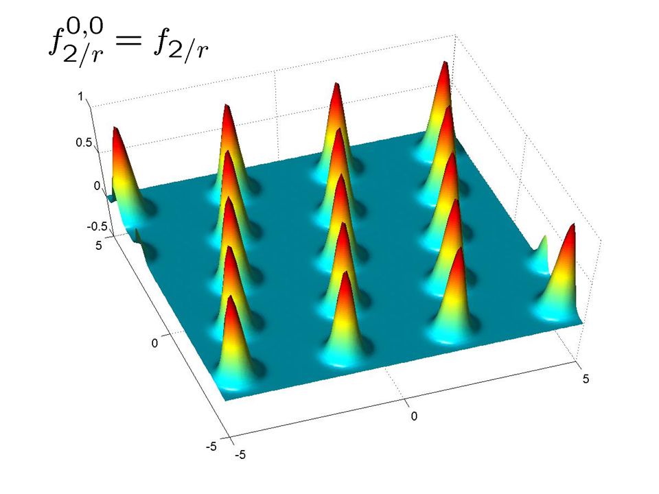
39. Approximating f 2/r Main idea: partition D r into 2 n distributions Main idea: partition D r into 2 n distributions For t  (Z 2 ) n, denote the translate t by D t r For t  (Z 2 ) n, denote the translate t by D t r Given a lattice point we can compute its t Given a lattice point we can compute its t The probability on (Z 2 ) n obtained by sampling from D r and outputting t is close to uniform The probability on (Z 2 ) n obtained by sampling from D r and outputting t is close to uniform 0,00,11,01,1

40. Hence, by using samples from D r we can produce samples from the following distribution on pairs (t,w): Hence, by using samples from D r we can produce samples from the following distribution on pairs (t,w): Sample t  Z 2 ) n uniformly at random Sample t  Z 2 ) n uniformly at random Sample w from D t r Sample w from D t r Consider the Fourier transform of D t r Consider the Fourier transform of D t r Approximating f 2/r

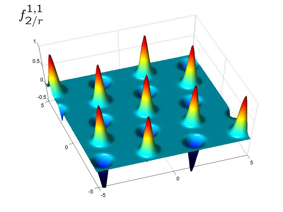
43. The functions f t 2/r look almost like f 2/r The functions f t 2/r look almost like f 2/r Only difference is that some Gaussians have their sign flipped Only difference is that some Gaussians have their sign flipped Approximating f t 2/r is enough: we can easily take the absolute value and obtain f 2/r Approximating f t 2/r is enough: we can easily take the absolute value and obtain f 2/r For this, however, we need to obtain several pairs (t,w) for the same t For this, however, we need to obtain several pairs (t,w) for the same t The problem is that each sample (t,w) has a different t ! The problem is that each sample (t,w) has a different t ! Approximating f 2/r

44. Fix x close to L * Fix x close to L * The sign of its Gaussian is ±1 depending on h s,t i mod 2 for s  (Z 2 ) n that depends only on x The sign of its Gaussian is ±1 depending on h s,t i mod 2 for s  (Z 2 ) n that depends only on x The distribution of  x,w  mod 2 when w is sampled from D t r is centred around  s,t  mod 2 The distribution of  x,w  mod 2 when w is sampled from D t r is centred around  s,t  mod 2 Hence, we obtain equations modulo 2 with error: Hence, we obtain equations modulo 2 with error: h s,t 1 i¼dh x,w 1 ic mod 2 h s,t 2 i¼dh x,w 2 ic mod 2 h s,t 3 i¼dh x,w 3 ic mod 2. Approximating f 2/r

45. Using the learning algorithm, we solve these equations and obtain s Using the learning algorithm, we solve these equations and obtain s Knowing s, we can cancel the sign Knowing s, we can cancel the sign Averaging over enough samples gives us an approximation to f 2/r Averaging over enough samples gives us an approximation to f 2/r Approximating f 2/r

46. Open Problems 1/4 Dequantize the reduction: Dequantize the reduction: This would lead to the ‘ultimate’ lattice- based cryptosystem (based on SVP, efficient) This would lead to the ‘ultimate’ lattice- based cryptosystem (based on SVP, efficient) Main obstacle: what can one do classically with a solution to CVP d ? Main obstacle: what can one do classically with a solution to CVP d ? Construct even more efficient schemes based on special classes of lattices such as cyclic lattices Construct even more efficient schemes based on special classes of lattices such as cyclic lattices For hash functions this was done by Micciancio For hash functions this was done by Micciancio

47. Open Problems 2/4 Extend to learning from parity (i.e., p=2) or even some constant p Extend to learning from parity (i.e., p=2) or even some constant p Is there something inherently different about the case of constant p? Is there something inherently different about the case of constant p? Use the ‘learning mod p’ problem to derive other lattice-based hardness results Use the ‘learning mod p’ problem to derive other lattice-based hardness results Recently, used by Klivans and Sherstov to derive hardness of learning problems Recently, used by Klivans and Sherstov to derive hardness of learning problems

48. Open Problems 3/4 Cryptanalysis Cryptanalysis Current attacks limited to low dimension [NguyenStern98] Current attacks limited to low dimension [NguyenStern98] New systems [Ajtai05,R05] are efficient and can be easily used with dimension 100+ New systems [Ajtai05,R05] are efficient and can be easily used with dimension 100+ Security against chosen-ciphertext attacks Security against chosen-ciphertext attacks Known lattice-based cryptosystems are not secure against CCA Known lattice-based cryptosystems are not secure against CCA

49. Open Problems 4/4 Comparison with number theoretic cryptography Comparison with number theoretic cryptography E.g., can one factor integers using an oracle for n-approximate SVP? E.g., can one factor integers using an oracle for n-approximate SVP? Signature schemes Signature schemes Can one construct provably secure lattice- based signature schemes? Can one construct provably secure lattice- based signature schemes?