Download presentation
Presentation is loading. Please wait.

1
Sample size calculation
Lecture on measures of disease occurence Ioannis Karagiannis based on previous EPIET material

2
Objectives: sample size
To understand: Why we estimate sample size Principles of sample size calculation Ingredients needed to estimate sample size

3
The idea of statistical inference
Generalisation to the population Conclusions based on the sample Population Hypotheses Sample

4
Why bother with sample size?
Pointless if power is too small Waste of resources if sample size needed is too large

5
Questions in sample size calculation
A national Salmonella outbreak has occurred with several hundred cases; You plan a case-control study to identify if consumption of food X is associated with infection; How many cases and controls should you recruit?

6
Questions in sample size calculation
An outbreak of 14 cases of a mysterious disease has occurred in cohort 2012; You suspect exposure to an activity is associated with illness and plan to undertake a cohort study under the kind auspices of coordinators; With the available cases, how much power will you have to detect a RR of 1.5?

7
Issues in sample size estimation
Estimate sample needed to measure the factor of interest Trade-off between study size and resources Sample size determined by various factors: significance level (α) power (1-β) expected prevalence of factor of interest
 power (1-β) expected prevalence of factor of interest.")
8
Which variables should be included in the sample size calculation?
The sample size calculation should relate to the study's primary outcome variable. If the study has secondary outcome variables which are also considered important, the sample size should also be sufficient for the analyses of these variables.

9
Allowing for response rates and other losses to the sample
The sample size calculation should relate to the final, achieved sample. Need to increase the initial numbers in accordance with: the expected response rate loss to follow up lack of compliance The link between the initial numbers approached and the final achieved sample size should be made explicit.

10
Significance testing: null and alternative hypotheses
Null hypothesis (H0) There is no difference Any difference is due to chance Alternative hypothesis (H1) There is a true difference
 There is no difference. Any difference is due to chance. Alternative hypothesis (H1) There is a true difference.")
11
Examples of null hypotheses
Case-control study H0: OR=1 “the odds of exposure among cases are the same as the odds of exposure among controls” Cohort study H0: RR=1 “the AR among the exposed is the same as the AR among the unexposed”

12
Significance level (p-value)
probability of finding a difference (RR≠1, reject H0), when no difference exists; α or type I error; usually set at 5%; p-value used to reject H0 (significance level); NB: a hypothesis is never “accepted”
, when no difference exists; α or type I error; usually set at 5%; p-value used to reject H0 (significance level); NB: a hypothesis is never accepted")
13
Type II error and power β is the type II error
probability of not finding a difference, when a difference really does exist Power is (1-β) and is usually set to 80% probability of finding a difference when a difference really does exist (=sensitivity)
 and is usually set to 80% probability of finding a difference when a difference really does exist (=sensitivity)")
14
Significance and power
Truth H0 true No difference H0 false Difference Decision Cannot reject H0 Correct decision Type II error = β Reject H0 Type I error level = α significance power = 1-β

15
How to increase power increase sample size
increase desired difference (or effect size) required NB: increasing the desired difference in RR/OR means move it away from 1! increase significance level desired (α error) Narrower confidence intervals
 required. NB: increasing the desired difference in RR/OR means move it away from 1! increase significance level desired (α error) Narrower confidence intervals.")
16
The effect of sample size
Consider 3 cohort studies looking at exposure to oysters with N=10, 100, 1000 In all 3 studies, 60% of the exposed are ill compared to 40% of unexposed (RR = 1.5)
")
17
Table A (N=10) Became ill Yes Total AR Ate oysters 3 5 3/5 No 2 2/5 10
5/10 RR=1.5, 95% CI: , p=0.53

18
Table B (N=100) Became ill Yes Total AR Ate oysters 30 50 30/50 No 20
20/50 100 50/100 RR=1.5, 95% CI: , p=0.046

19
Table C (N=1000) Became ill Yes No AR Ate oysters 300 500 300/500 200
200/500 Total 1000 500/1000 RR=1.5, 95% CI: , p<0.001

20
Sample size and power In Table A, with n=10 sample, there was no significant association with oysters, but there was with a larger sample size. In Tables B and C, with bigger samples, the association became significant.

21
Cohort sample size: parameters to consider
Risk ratio worth detecting Expected frequency of disease in unexposed population Ratio of unexposed to exposed Desired level of significance (α) Power of the study (1-β)
 Power of the study (1-β)")
22
Cohort: Episheet Power calculation
Risk of α error % Population exposed Exp freq disease in unexposed 5% Ratio of unexposed to exposed 1:1 RR to detect ≥1.5 The power of a statistical test is the probability that the test will reject a false null hypothesis, or in other words that it will not make a Type II error. The higher the power, the greater the chance of obtaining a statistically significant result when the null hypothesis is false. Statistical power depends on the significance criterion, the size of the difference or the strength of the similarity (that is, the effect size) in the population, and the sensitivity of the data.
 in the population, and the sensitivity of the data.")
25
Case-control sample size: parameters to consider
Number of cases Number of controls per case OR ratio worth detecting % of exposed persons in source population Desired level of significance (α) Power of the study (1-β)
 Power of the study (1-β)")
26
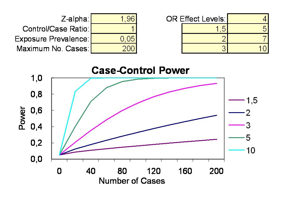
Case-control: Power calculation
α error % Number of cases Proportion of controls exposed 5% OR to detect ≥1.5 No. controls/case 1:1 The power of a statistical test is the probability that the test will reject a false null hypothesis, or in other words that it will not make a Type II error. The higher the power, the greater the chance of obtaining a statistically significant result when the null hypothesis is false. Statistical power depends on the significance criterion, the size of the difference or the strength of the similarity (that is, the effect size) in the population, and the sensitivity of the data.
 in the population, and the sensitivity of the data.")
28
Statistical Power of a Case-Control Study for different control-to-case ratios and odds ratios (50 cases) a probability is a number between 0 and 1; the probability of an event or proposition and its complement must add up to 1; and the joint probability of two events or propositions is the product of the probability of one of them and the probability of the second, conditional on the first. Representation and interpretation of probability values The probability of an event is generally represented as a real number between 0 and 1, inclusive. An impossible event has a probability of exactly 0, and a certain event has a probability of 1, but the converses are not always true: probability 0 events are not always impossible, nor probability 1 events certain. The rather subtle distinction between "certain" and "probability 1" is treated at greater length in the article on "almost surely". Most probabilities that occur in practice are numbers between 0 and 1, indicating the event's position on the continuum between impossibility and certainty. The closer an event's probability is to 1, the more likely it is to occur. For example, if two mutually exclusive events are assumed equally probable, such as a flipped coin landing heads-up or tails-up, we can express the probability of each event as "1 in 2", or, equivalently, "50%" or "1/2". Probabilities are equivalently expressed as odds, which is the ratio of the probability of one event to the probability of all other events. The odds of heads-up, for the tossed coin, are (1/2)/(1 - 1/2), which is equal to 1/1. This is expressed as "1 to 1 odds" and often written "1:1". Odds a:b for some event are equivalent to probability a/(a+b). For example, 1:1 odds are equivalent to probability 1/2, and 3:2 odds are equivalent to probability 3/5. There remains the question of exactly what can be assigned probability, and how the numbers so assigned can be used; this is the question of probability interpretations.
/(1 - 1/2), which is equal to 1/1. This is expressed as 1 to 1 odds and often written 1:1 . Odds a:b for some event are equivalent to probability a/(a+b). For example, 1:1 odds are equivalent to probability 1/2, and 3:2 odds are equivalent to probability 3/5. There remains the question of exactly what can be assigned probability, and how the numbers so assigned can be used; this is the question of probability interpretations.")
29
Statistical Power of a Case-Control Study

30
Sample size for proportions: parameters to consider
Population size Anticipated p α error Design effect Easy to calculate on openepi.com

31
Conclusions Don’t forget to undertake sample size/power calculations
Use all sources of currently available data to inform your estimates Try several scenarios Adjust for non-response Let it be feasible

32
Acknowledgements Nick Andrews, Richard Pebody, Viviane Bremer

Similar presentations


 18 th EPIET/EUPHEM Introductory course 28.09.2012.>")


 Is a tests ability to detect a false hypothesis Is the probability that.>")


 www.ahrq.gov.>")


