Download presentation
Presentation is loading. Please wait.

1
The Variability of Sea Ice from Aqua’s AMSR-E Instrument: A Quantitative Comparison of the Team and Bootstrap Algorithms By Lorraine M. Beane Dr. Claire L. Parkinson, advisor Research and Discover Program August 12, 2004 (Image courtesy of NOAA) Supported by the Research and Discover Program
 Supported by the Research and Discover Program.")
2
Sea Ice Formed by the freezing of sea water –As freezing occurs, some of the salt drops down, leaving a layer of higher salinity water underneath the less saline ice (first year ice salinity is 10 ppt, multiyear ice salinity is 3 ppt) Found primarily in Arctic and Antarctic regions Spreads over approximately 25 million km 2 Growth in the first year can be 1-2 meters, although typically does not reach thicknesses of > 5 meters Average lifespan is 3-5 years
 Found primarily in Arctic and Antarctic regions Spreads over approximately 25 million km 2 Growth in the first year can be 1-2 meters, although typically does not reach thicknesses of > 5 meters Average lifespan is 3-5 years")
3
Sea Ice Impacts on Climate Change Insulator of oceans at high latitudes –Feedback effects Highly reflective surface reduces amount of absorbed solar radiation Affects much of the Earth’s deep ocean waters due to salt release –Stratification of the oceans –Global circulation patterns General trends since late 1978 show that sea ice is decreasing in the Arctic and increasing in the Antarctic The GCM at NASA Goddard Institute for Space Studies (GISS) indicates that as much as 37% of simulated global temperature rise is due to sea ice changes and the feedback effects they have on the rest of the system (Rind et al., 1995) from C. Parkinson, D. Cavalieri, J. Comiso, P. Gloersen, and J. Zwally

4
Sea Ice Observation Monitoring of sea ice is possible in the visible spectrum, but is often problematic due to cloud cover and darkness –This obstacle is overcome by using the microwave portion of the EM spectrum –Brightness temperature is a measure of radiation in temperature units Record is extensive and nearly continuous –Began in December 1972; most complete since late October 1978 –Most recent data is from the Aqua spacecraft www.thinkquest.org

5
Aqua Launched on May 4, 2002 into a near polar orbit –Sea ice observation carried out using the Advanced Microwave Scanning Radiometer (AMSR-E) Developed by Mitsubishi Electric Corporation under a contract from the National Space Development Agency of Japan (NASDA), subsequently merged into the Japan Aerospace Exploration Agency (JAXA) Passive microwave radiometer Two products are developed from this raw data to determine sea ice concentration using algorithms http://aqua.gsfc.nasa.gov
 Developed by Mitsubishi Electric Corporation under a contract from the National Space Development Agency of Japan (NASDA), subsequently merged into the Japan Aerospace Exploration Agency (JAXA) Passive microwave radiometer Two products are developed from this raw data to determine sea ice concentration using algorithms")
6
Algorithms Two products are the ice coverages given by the Team and Bootstrap algorithms –Team is the standard in the Arctic –Bootstrap is standard in the Antarctic Used to determine sea ice concentration and extent…not thickness Both use the 19 GHz and 37 GHz frequencies –Team also uses 85 GHz –Bootstrap also uses 6 GHz Each uses different reference brightness temperatures, channel combinations, and weather filters

7
Goals of Research To conduct a quantitative investigation into the differences between the Team and Bootstrap algorithm results –Where do they differ? –How do they differ? –Are there differences in their behavior between the two poles? –Are there any trends in their behavior?

8
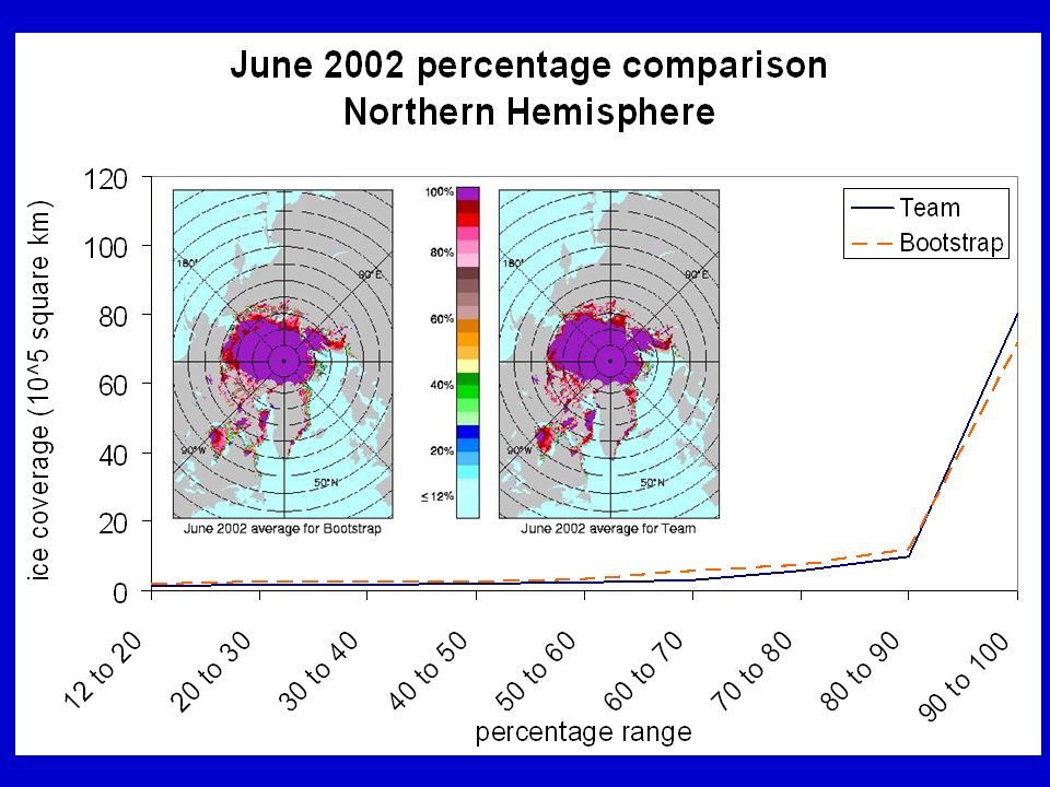
June 2002 Northern Hemisphere

9
June 2002 differences in the Northern Hemisphere Team – Bootstrap Percent difference (%) # of hits
 # of hits")
10
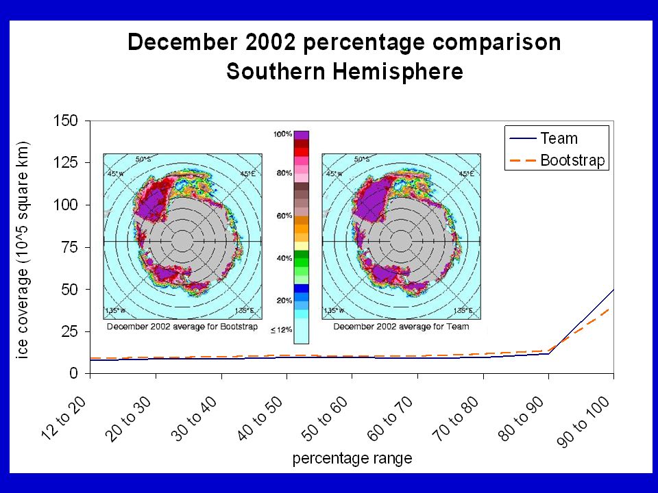
December 2002 Southern Hemisphere

11
December 2002 differences in the Southern Hemisphere Percent difference (%) # of hits Team - Bootstrap
 # of hits Team - Bootstrap")
12
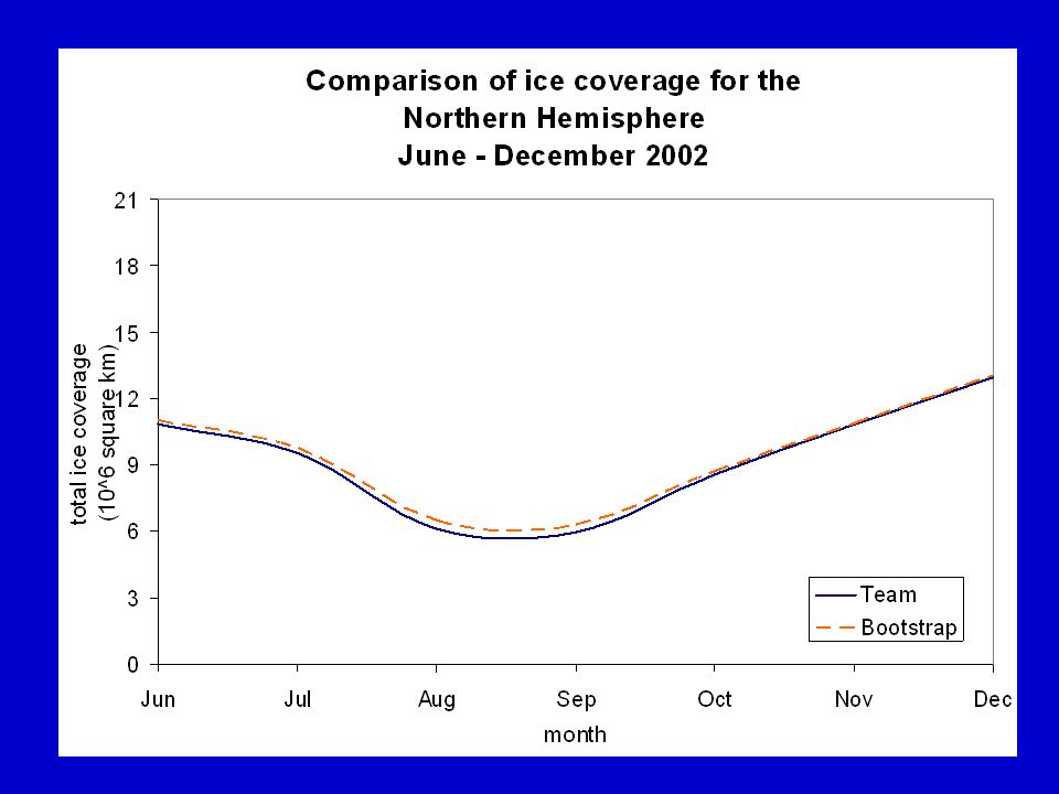
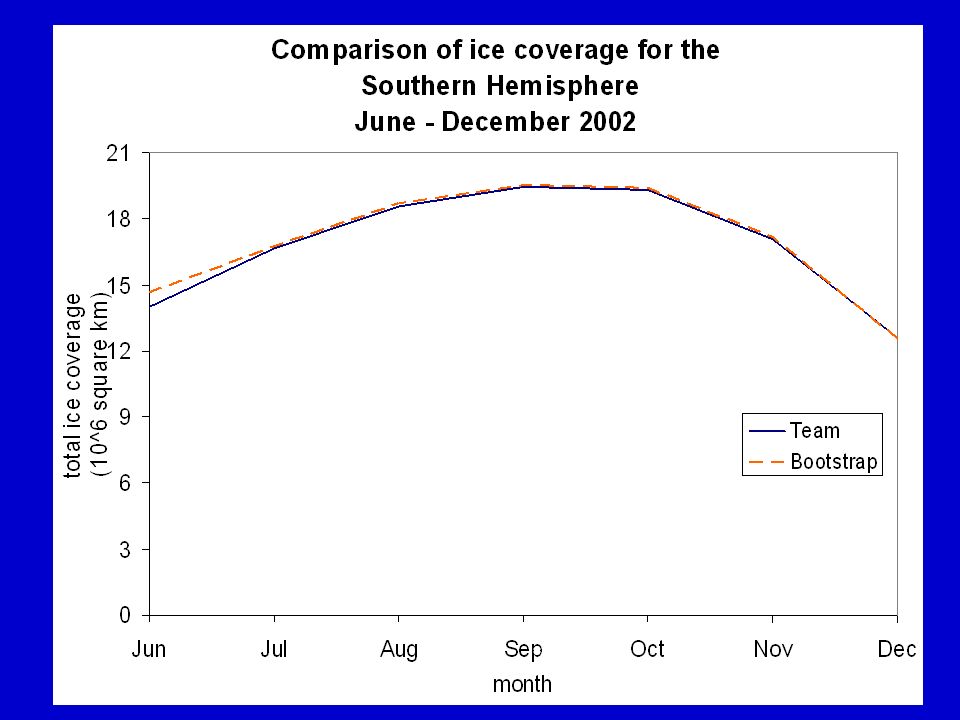
Seasonal Variability of Sea Ice for 2002

17
Conclusions Overall, both algorithms show very similar sea ice coverage, with the Bootstrap yielding slightly higher total ice coverage for the months examined Most often the Bootstrap algorithm shows a more extensive coverage at lower concentrations and a less extensive coverage at the 90-100% range

18
More Conclusions In the Northern Hemisphere –The Bootstrap yields higher concentrations over the majority of the region, typically <10% difference –The Team yields higher concentrations over the peripheral regions with differences up to around 20% In the Southern Hemisphere –The Team gives concentrations of 2-10% higher for a large portion of the hemisphere –Occasionally the Bootstrap shows higher concentrations along the edges of the ice and also in the Weddell and Ross seas, at least in the months examined

19
Further Analysis Completion of reprocessing of data in order to complete this analysis for an entire year –Seasonal variations –Comparisons of the same seasons at opposite poles (i.e. summer in the Arctic versus summer in the Antarctic) Validation from the field –Efforts underway for both hemispheres, primarily via aircraft flyovers Arctic campaigns 2002-2005 Antarctic campaign scheduled for September 2004
 Validation from the field –Efforts underway for both hemispheres, primarily via aircraft flyovers Arctic campaigns Antarctic campaign scheduled for September")
20
Thanks and Acknowledgements Dr. Claire L. Parkinson Nick DiGirolamo Dr. Donald J. Cavalieri and Alvaro Ivanhoff Dr. Josefino C. Comiso and Rob Gersten Dr. George Hurtt and Dr. Vince Salomonson of the Research and Discover Program NASA Goddard Space Flight Center University of New Hampshire

Similar presentations


 THE ARCTIC’S RAPIDLY SHRINKING SEA ICE COVER: A RESEARCH SYNTHESIS PRESENTATION Zachary Looney 2 nd Year Atmospheric Sciences>")


 Menglin Jin, San Jose Stte University Outline Physical principles International satellite.>")


