1. Multivariate Analysis

2. One-way ANOVA Tests the difference in the means of 2 or more nominal groups Tests the difference in the means of 2 or more nominal groups E.g., High vs. Medium vs. Low exposure E.g., High vs. Medium vs. Low exposure Can be used with more than one IV Can be used with more than one IV Two-way ANOVA, Three-way ANOVA etc. Two-way ANOVA, Three-way ANOVA etc.

3. ANOVA _______-way ANOVA _______-way ANOVA Number refers to the number of IVs Number refers to the number of IVs Tests whether there are differences in the means of IV groups Tests whether there are differences in the means of IV groups E.g.: E.g.: Experimental vs. control group Experimental vs. control group Women vs. Men Women vs. Men High vs. Medium vs. Low exposure High vs. Medium vs. Low exposure

4. Logic of ANOVA Variance partitioned into: Variance partitioned into: 1. Systematic variance: 1. Systematic variance: the result of the influence of the Ivs the result of the influence of the Ivs 2. Error variance: 2. Error variance: the result of unknown factors the result of unknown factors Variation in scores partitions the variance into two parts by calculating the “sum of squares”: Variation in scores partitions the variance into two parts by calculating the “sum of squares”: 1. Between groups variation (systematic) 1. Between groups variation (systematic) 2. Within groups variation (error) 2. Within groups variation (error) SS total = SS between + SS within SS total = SS between + SS within

5. Significant and Non-significant Differences Significant: Between > Within Non-significant: Within > Between

6. Partitioning the Variance Comparisons Total variation = score – grand mean Total variation = score – grand mean Between variation = group mean – grand mean Between variation = group mean – grand mean Within variation = score – group mean Within variation = score – group mean Deviation is taken, then squared, then summed across cases Deviation is taken, then squared, then summed across cases Hence the term “Sum of squares” (SS) Hence the term “Sum of squares” (SS)

7. One-way ANOVA example Total SS (deviation from grand mean) Group AGroup BGroup C 49 56 54 52 57 52 52 57 56 53 60 50 49 60 53 Mean = 51 58 53 Grand mean = 54

8. One-way ANOVA example Total SS (deviation from grand mean) Group A Group B Group C -5 25 2 4 0 0 -2 4 3 9 -2 4 -2 4 3 9 2 4 -1 1 636 -416 -5 25 636 -1 1 Sum of squares = 59 + 94 + 25 = 178

9. One-way ANOVA example Between SS (group mean – grand mean) A B C Group means515853 Group deviation from grand mean-3 4-1 Squared deviation 916 1 n(squared deviation)4580 5 Between SS = 45 + 80 + 5 = 130 Grand mean = 54

10. One-way ANOVA example Within SS (score - group mean) ABC 515853 Deviation from group means -2 -21 1-1-1 1-1 3 2 2-3 -2 2 0 Squared deviations4 4 1 111 119 449 440 Within SS = 14 + 14 + 20 = 48

11. The F equation for ANOVA F = Between groups sum of squares/(k-1) Within groups sum of squares/(N-k) Within groups sum of squares/(N-k) N = total number of subjects k = number of groups Numerator = Mean square between groups Denominator = Mean square within groups

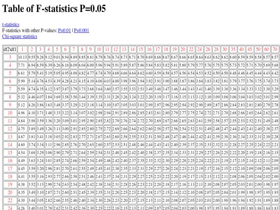
13. Significance of F F-critical is 3.89 (2,12 df) F observed 16.25 > F critical 3.89 Groups are significantly different -T-tests could then be run to determine which groups are significantly different from which other groups

14. Computer Printout Example

15. Two-way ANOVA ANOVA compares: ANOVA compares: Between and within groups variance Between and within groups variance Adds a second IV to one-way ANOVA Adds a second IV to one-way ANOVA 2 IV and 1 DV 2 IV and 1 DV Analyzes significance of: Analyzes significance of: Main effects of each IV Main effects of each IV Interaction effect of the IVs Interaction effect of the IVs

16. Graphs of potential outcomes No main effects or interactions No main effects or interactions Main effects of color only Main effects of color only Main effects for motion only Main effects for motion only Main effects for color and motion Main effects for color and motion Interactions Interactions

17. Graphs Color B&W x Motion * Still AROUSALAROUSAL

18. No main effects for interactions Color B&W x Motion * Still AROUSALAROUSAL

19. No main effects for interactions Color B&W x Motion * Still x x * * AROUSALAROUSAL

20. Main effects for color only Color B&W x Motion * Still AROUSALAROUSAL

21. Main effects for color only Color B&W x Motion * Still x x * * AROUSALAROUSAL

22. Main effects for motion only Color B&W x Motion * Still AROUSALAROUSAL

23. Main effects for motion only Color B&W x Motion * Still x x ** AROUSALAROUSAL

24. Main effects for color and motion Color B&W x Motion * Still AROUSALAROUSAL

25. Main effects for color and motion Color B&W x Motion * Still x x * * AROUSALAROUSAL

26. Transverse interaction Color B&W x Motion * Still AROUSALAROUSAL

27. Transverse interaction Color B&W x Motion * Still x x * * AROUSALAROUSAL

28. Interaction—color only makes a difference for motion Color B&W x Motion * Still AROUSALAROUSAL

29. Interaction—color only makes a difference for motion Color B&W x Motion * Still x x * * AROUSALAROUSAL

30. Partitioning the variance for Two- way ANOVA Total variation = Main effect variable 1 + Main effect variable 2 + Interaction + Residual (within)

31. Summary Table for Two-way ANOVA SourceSSdfMSF Main effect 1 Main effect 2 InteractionWithinTotal

32. Printout Example

33. Printout plot

34. Scatter Plot of Price and Attendance Price is the average seat price for a single regular season game in today’s dollars Price is the average seat price for a single regular season game in today’s dollars Attendance is total annual attendance and is in millions of people per annum. Attendance is total annual attendance and is in millions of people per annum.

35. Is there a relation there? Lets use linear regression to find out, that is Lets use linear regression to find out, that is Let’s fit a straight line to the data. Let’s fit a straight line to the data. But aren’t there lots of straight lines that could fit? But aren’t there lots of straight lines that could fit? Yes! Yes!

36. Desirable Properties We would like the “closest” line, that is the one that minimizes the error We would like the “closest” line, that is the one that minimizes the error The idea here is that there is actually a relation, but there is also noise. We would like to make sure the noise (i.e., the deviation from the postulated straight line) to be as small as possible. The idea here is that there is actually a relation, but there is also noise. We would like to make sure the noise (i.e., the deviation from the postulated straight line) to be as small as possible. We would like the error (or noise) to be unrelated to the independent variable (in this case price). We would like the error (or noise) to be unrelated to the independent variable (in this case price). If it were, it would not be noise --- right! If it were, it would not be noise --- right!

37. Scatter Plot of Price and Attendance Price is the average seat price for a single regular season game in today’s dollars Price is the average seat price for a single regular season game in today’s dollars Attendance is total annual attendance and is in millions of people per annum. Attendance is total annual attendance and is in millions of people per annum.

38. Simple Regression The simple linear regression MODEL is: The simple linear regression MODEL is: y =  0 +  1 x +  describes how y is related to x describes how y is related to x  0 and  1 are called parameters of the model.  0 and  1 are called parameters of the model.  is a random variable called the error term.  is a random variable called the error term. xy e

39. Simple Regression Graph of the regression equation is a straight line. Graph of the regression equation is a straight line. β is the population y-intercept of the regression line. β 0 is the population y-intercept of the regression line. β 1 is the population slope of the regression line. β 1 is the population slope of the regression line. E(y) is the expected value of y for a given x value E(y) is the expected value of y for a given x value

40. Simple Regression E(y)E(y)E(y)E(y) x Slope  1 is positive Regression line Intercept  0

41. Simple Regression E(y)E(y)E(y)E(y) x Slope  1 is 0 Regression line Intercept  0

42. Types of Regression Models

43. Regression Modeling Steps 1.Hypothesize Deterministic Components 1.Hypothesize Deterministic Components 2.Estimate Unknown Model Parameters 2.Estimate Unknown Model Parameters 3.Specify Probability Distribution of Random Error Term 3.Specify Probability Distribution of Random Error Term Estimate Standard Deviation of Error Estimate Standard Deviation of Error 4.Evaluate Model 4.Evaluate Model 5.Use Model for Prediction & Estimation 5.Use Model for Prediction & Estimation

44. Linear Multiple Regression Model 1.Relationship between 1 dependent & 2 or more independent variables is a linear function 1.Relationship between 1 dependent & 2 or more independent variables is a linear function Dependent (response) variable Independent (explanatory) variables Population slopes Population Y-intercept Random error

45. Multiple Regression Model Multivariate model