Download presentation
Presentation is loading. Please wait.

1
Statistics for Business and Economics
Chapter 10 Simple Linear Regression

2
Learning Objectives Describe the Linear Regression Model
State the Regression Modeling Steps Explain Least Squares Compute Regression Coefficients Explain Correlation Predict Response Variable As a result of this class, you will be able to...

3
Models

4
Models Representation of some phenomenon
Mathematical model is a mathematical expression of some phenomenon Often describe relationships between variables Types Deterministic models Probabilistic models .

5
Deterministic Models Hypothesize exact relationships
Suitable when prediction error is negligible Example: force is exactly mass times acceleration F = m·a © T/Maker Co.

6
Probabilistic Models Hypothesize two components
Deterministic Random error Example: sales volume (y) is 10 times advertising spending (x) + random error y = 10x + Random error may be due to factors other than advertising
 is 10 times advertising spending (x) + random error. y = 10x + Random error may be due to factors other than advertising.")
7
Types of Probabilistic Models
Regression Models Correlation Models 7

8
Regression Models

9
Types of Probabilistic Models
Regression Models Correlation Models 7

10
Regression Models Answers ‘What is the relationship between the variables?’ Equation used One numerical dependent (response) variable What is to be predicted One or more numerical or categorical independent (explanatory) variables Used mainly for prediction and estimation
 variables. Used mainly for prediction and estimation.")
11
Regression Modeling Steps
Hypothesize deterministic component Estimate unknown model parameters Specify probability distribution of random error term Estimate standard deviation of error Evaluate model Use model for prediction and estimation

12
Model Specification

13
Regression Modeling Steps
Hypothesize deterministic component Estimate unknown model parameters Specify probability distribution of random error term Estimate standard deviation of error Evaluate model Use model for prediction and estimation

14
Specifying the Model Define variables
Conceptual (e.g., Advertising, price) Empirical (e.g., List price, regular price) Measurement (e.g., $, Units) Hypothesize nature of relationship Expected effects (i.e., Coefficients’ signs) Functional form (linear or non-linear) Interactions
 Empirical (e.g., List price, regular price) Measurement (e.g., $, Units) Hypothesize nature of relationship. Expected effects (i.e., Coefficients’ signs) Functional form (linear or non-linear) Interactions.")
15
Model Specification Is Based on Theory
Theory of field (e.g., Sociology) Mathematical theory Previous research ‘Common sense’
 Mathematical theory. Previous research. ‘Common sense’")
16
Thinking Challenge: Which Is More Logical?
Sales Sales With positive linear relationship, sales increases infinitely. Discuss concept of ‘relevant range’. Advertising Advertising Sales Sales Advertising Advertising 17

17
Types of Regression Models
Simple 1 Explanatory Variable 2+ Explanatory Variables Multiple This teleology is based on the number of explanatory variables & nature of relationship between X & Y. Linear Non- Linear Linear Non- Linear 19

18
Linear Regression Model

19
Types of Regression Models
Simple 1 Explanatory Variable Regression Models 2+ Explanatory Variables Multiple Linear Non- This teleology is based on the number of explanatory variables & nature of relationship between X & Y. 27

20
Linear Regression Model
Relationship between variables is a linear function Population y-intercept Population Slope Random Error y x 1 Dependent (Response) Variable Independent (Explanatory) Variable
 Variable. Independent (Explanatory) Variable.")
21
Line of Means y x E(y) = β0 + β1x (line of means) Change in y
β1 = Slope Change in x β0 = y-intercept x 28

22
Population & Sample Regression Models
Random Sample $ Unknown Relationship $ $ $ $ $ 31

23
Population Linear Regression Model
y Observed value i = Random error x Observed value 35

24
Sample Linear Regression Model
y i = Random error ^ Unsampled observation x Observed value 36

25
Estimating Parameters: Least Squares Method

26
Regression Modeling Steps
Hypothesize deterministic component Estimate unknown model parameters Specify probability distribution of random error term Estimate standard deviation of error Evaluate model Use model for prediction and estimation

27
Scattergram Plot of all (xi, yi) pairs
Suggests how well model will fit 20 40 60 x y

28
Thinking Challenge How would you draw a line through the points?
How do you determine which line ‘fits best’? 20 40 60 x y 42

29
Least Squares ‘Best fit’ means difference between actual y values and predicted y values are a minimum But positive differences off-set negative Least Squares minimizes the Sum of the Squared Differences (SSE) 49
 49.")
30
Least Squares Graphically
^ e ^ 4 2 ^ e e ^ 1 3 x 52

31
Coefficient Equations
Prediction Equation Slope y-intercept 53

32
Computation Table xi yi xi yi xiyi x1 y1 x1 y1 x1y1 x2 y2 x2 y2 x2y2 :
xn yn xn 2 yn xnyn 2 2 Σxi Σyi Σxi Σyi Σxiyi 54

33
Interpretation of Coefficients
^ Slope (1) Estimated y changes by 1 for each 1unit increase in x If 1 = 2, then Sales (y) is expected to increase by 2 for each 1 unit increase in Advertising (x) Y-Intercept (0) Average value of y when x = 0 If 0 = 4, then Average Sales (y) is expected to be 4 when Advertising (x) is 0 ^
 Estimated y changes by 1 for each 1unit increase in x. If 1 = 2, then Sales (y) is expected to increase by 2 for each 1 unit increase in Advertising (x) Y-Intercept (0) Average value of y when x = 0. If 0 = 4, then Average Sales (y) is expected to be 4 when Advertising (x) is 0. ^")
34
Least Squares Example You’re a marketing analyst for Hasbro Toys. You gather the following data: Ad $ Sales (Units) Find the least squares line relating sales and advertising.

35
Scattergram Sales vs. Advertising
4 3 2 1 1 2 3 4 5 Advertising 57

36
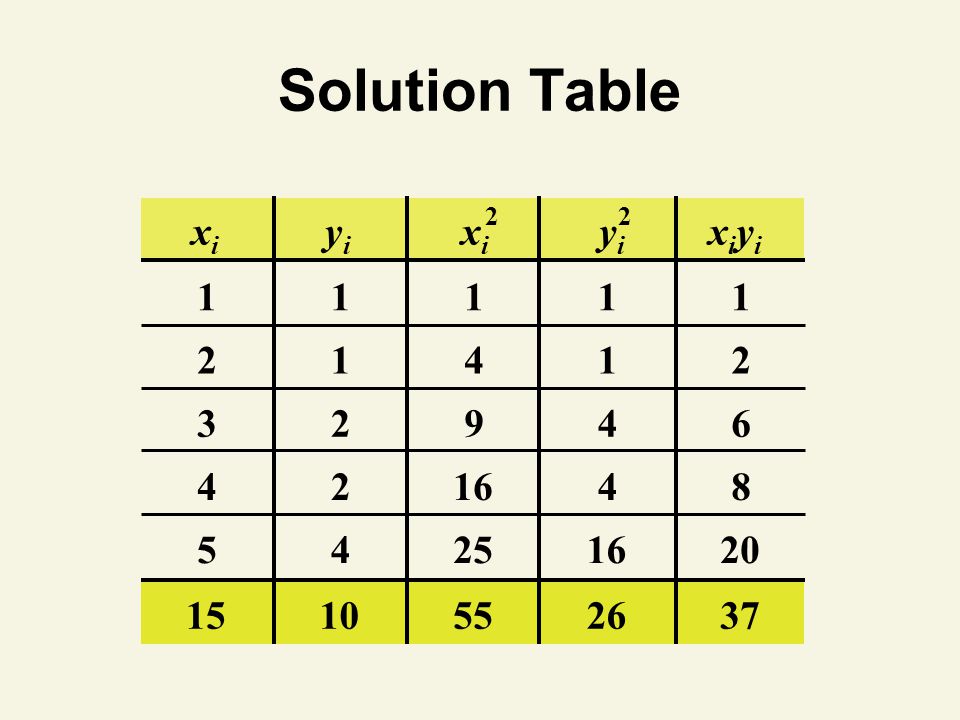
Parameter Estimation Solution Table
xi yi xi 2 yi 2 xiyi 1 1 1 1 1 2 1 4 1 2 3 2 9 4 6 4 2 16 4 8 5 4 25 16 20 15 10 55 26 37 58

37
Parameter Estimation Solution
59

38
Parameter Estimation Computer Output
Parameter Estimates Parameter Standard T for H0: Variable DF Estimate Error Param=0 Prob>|T| INTERCEP ADVERT ^ 0 ^ 1

39
Coefficient Interpretation Solution
Slope (1) Sales Volume (y) is expected to increase by .7 units for each $1 increase in Advertising (x) ^ Y-Intercept (0) Average value of Sales Volume (y) is -.10 units when Advertising (x) is 0 Difficult to explain to marketing manager Expect some sales without advertising ^
 Sales Volume (y) is expected to increase by .7 units for each $1 increase in Advertising (x) ^ Y-Intercept (0) Average value of Sales Volume (y) is -.10 units when Advertising (x) is 0. Difficult to explain to marketing manager. Expect some sales without advertising. ^")
40
Regression Line Fitted to the Data
Sales 4 3 2 1 1 2 3 4 5 Advertising 57

41
Least Squares Thinking Challenge
You’re an economist for the county cooperative. You gather the following data: Fertilizer (lb.) Yield (lb.) Find the least squares line relating crop yield and fertilizer. © T/Maker Co. 62
 Yield (lb.) Find the least squares line relating crop yield and fertilizer. © T/Maker Co. 62.")
42
Scattergram Crop Yield vs. Fertilizer*
Yield (lb.) 10 8 6 4 2 5 10 15 Fertilizer (lb.) 65
 Fertilizer (lb.) 65.")
43
Parameter Estimation Solution Table*
2 2 xi yi xi yi xiyi 4 3.0 16 9.00 12 6 5.5 36 30.25 33 10 6.5 100 42.25 65 12 9.0 144 81.00 108 32 24.0 296 162.50 218 66

44
Parameter Estimation Solution*
67

45
Coefficient Interpretation Solution*
^ Slope (1) Crop Yield (y) is expected to increase by .65 lb. for each 1 lb. increase in Fertilizer (x) Y-Intercept (0) Average Crop Yield (y) is expected to be 0.8 lb. when no Fertilizer (x) is used ^
 Crop Yield (y) is expected to increase by .65 lb. for each 1 lb. increase in Fertilizer (x) Y-Intercept (0) Average Crop Yield (y) is expected to be 0.8 lb. when no Fertilizer (x) is used. ^")
46
Regression Line Fitted to the Data*
Yield (lb.) 10 8 6 4 2 5 10 15 Fertilizer (lb.) 65
 Fertilizer (lb.) 65.")
47
Probability Distribution of Random Error

48
Regression Modeling Steps
Hypothesize deterministic component Estimate unknown model parameters Specify probability distribution of random error term Estimate standard deviation of error Evaluate model Use model for prediction and estimation

49
Linear Regression Assumptions
Mean of probability distribution of error, ε, is 0 Probability distribution of error has constant variance Probability distribution of error, ε, is normal Errors are independent

50
Error Probability Distribution
E(y) = β0 + β1x x x1 x2 x3 91
 = β0 + β1x. x. x1. x2. x")
51
Random Error Variation
^ Variation of actual y from predicted y, y Measured by standard error of regression model Sample standard deviation of : s ^ Affects several factors Parameter significance Prediction accuracy

52
Variation Measures y x xi yi y Unexplained sum of squares
Total sum of squares Explained sum of squares y x xi 78

53
Estimation of σ2

54
Calculating SSE, s2, s Example
You’re a marketing analyst for Hasbro Toys. You gather the following data: Ad $ Sales (Units) Find SSE, s2, and s.
 Find SSE, s2, and s.")
55
Calculating SSE Solution
xi yi 1 1 .6 .4 .16 2 1 1.3 -.3 .09 3 2 2 4 2 2.7 -.7 .49 5 4 3.4 .6 .36 SSE=1.1

56
Calculating s2 and s Solution

57
Testing for Significance
Evaluating the Model Testing for Significance

58
Regression Modeling Steps
Hypothesize deterministic component Estimate unknown model parameters Specify probability distribution of random error term Estimate standard deviation of error Evaluate model Use model for prediction and estimation

59
Test of Slope Coefficient
Shows if there is a linear relationship between x and y Involves population slope 1 Hypotheses H0: 1 = 0 (No Linear Relationship) Ha: 1 0 (Linear Relationship) Theoretical basis is sampling distribution of slope
 Ha: 1 0 (Linear Relationship) Theoretical basis is sampling distribution of slope.")
60
Sampling Distribution of Sample Slopes
y Sample 1 Line All Possible Sample Slopes Sample 1: 2.5 Sample 2: 1.6 Sample 3: 1.8 Sample 4: : : Very large number of sample slopes Sample 2 Line Population Line x b 1 Sampling Distribution 1 S ^ 105

61
Slope Coefficient Test Statistic
106

62
Test of Slope Coefficient Example
You’re a marketing analyst for Hasbro Toys. You find β0 = –.1, β1 = .7 and s = Ad $ Sales (Units) Is the relationship significant at the .05 level of significance? ^ ^
 Is the relationship significant at the .05 level of significance ^ ^")
63
Test of Slope Coefficient Solution
H0: Ha: df Critical Value(s): 1 = 0 1 0 Test Statistic: Decision: Conclusion: .05 5 - 2 = 3 t 3.182 -3.182 .025 Reject H0 109
: 1 = 0. 1 0. Test Statistic: Decision: Conclusion: = 3. t Reject H")
64
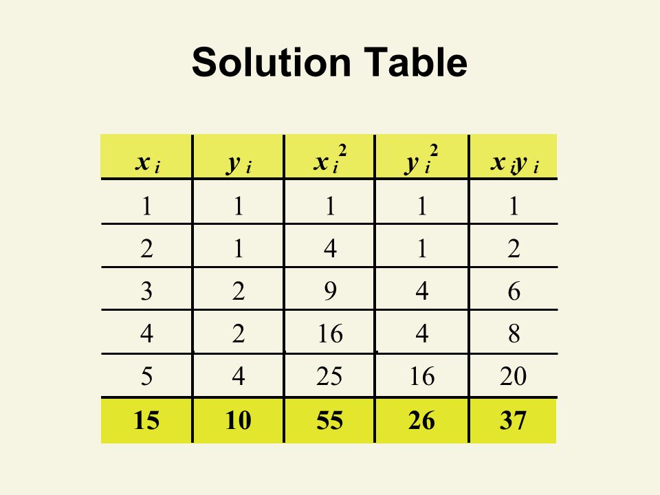
Solution Table xi yi xi yi xiyi 1 1 1 1 1 2 1 4 1 2 3 2 9 4 6 4 2 16 4
8 5 4 25 16 20 15 10 55 26 37 108

65
Test Statistic Solution

66
Test of Slope Coefficient Solution
H0: 1 = 0 Ha: 1 0 .05 df = 3 Critical Value(s): Test Statistic: Decision: Conclusion: t 3.182 -3.182 .025 Reject H0 Reject at = .05 There is evidence of a relationship 109
: Test Statistic: Decision: Conclusion: t Reject H0. Reject at = .05. There is evidence of a relationship")
67
Test of Slope Coefficient Computer Output
Parameter Estimates Parameter Standard T for H0: Variable DF Estimate Error Param=0 Prob>|T| INTERCEP ADVERT ‘Standard Error’ is the estimated standard deviation of the sampling distribution, sbP. ^ ^ S ^ t = 1 / S 1 ^ 1 1 P-Value

68
Correlation Models

69
Types of Probabilistic Models
Regression Models Correlation Models 130

70
Correlation Models Answers ‘How strong is the linear relationship between two variables?’ Coefficient of correlation Sample correlation coefficient denoted r Values range from –1 to +1 Measures degree of association Does not indicate cause–effect relationship

71
Coefficient of Correlation
where

72
Coefficient of Correlation Values
Perfect Negative Correlation Perfect Positive Correlation No Linear Correlation –1.0 –.5 +.5 +1.0 Increasing degree of negative correlation Increasing degree of positive correlation 134

73
Coefficient of Correlation Example
You’re a marketing analyst for Hasbro Toys. Ad $ Sales (Units) Calculate the coefficient of correlation. 83
 Calculate the coefficient of correlation. 83.")
74
Solution Table xi yi xi yi xiyi 1 1 1 1 1 2 1 4 1 2 3 2 9 4 6 4 2 16 4
8 5 4 25 16 20 15 10 55 26 37 108
75
Coefficient of Correlation Solution

76
Coefficient of Correlation Thinking Challenge
You’re an economist for the county cooperative. You gather the following data: Fertilizer (lb.) Yield (lb.) Find the coefficient of correlation. © T/Maker Co. 62
 Yield (lb.) Find the coefficient of correlation. © T/Maker Co. 62.")
77
Solution Table* xi yi xi yi xiyi 4 3.0 16 9.00 12 6 5.5 36 30.25 33 10
6.5 100 42.25 65 12 9.0 144 81.00 108 32 24.0 296 162.50 218 66

78
Coefficient of Correlation Solution*

79
Coefficient of Determination
Proportion of variation ‘explained’ by relationship between x and y 0 r2 1 r2 = (coefficient of correlation)2 79
")
80
Coefficient of Determination Example
You’re a marketing analyst for Hasbro Toys. You know r = .904. Ad $ Sales (Units) Calculate and interpret the coefficient of determination. 83
 Calculate and interpret the coefficient of determination. 83.")
81
Coefficient of Determination Solution
r2 = (coefficient of correlation)2 r2 = (.904)2 r2 = .817 Interpretation: About 81.7% of the sample variation in Sales (y) can be explained by using Ad $ (x) to predict Sales (y) in the linear model. 83
2. r2 = (.904)2. r2 = Interpretation: About 81.7% of the sample variation in Sales (y) can be explained by using Ad $ (x) to predict Sales (y) in the linear model. 83.")
82
r2 Computer Output Root MSE R-square Dep Mean Adj R-sq C.V r2 r2 adjusted for number of explanatory variables & sample size

83
Using the Model for Prediction & Estimation

84
Regression Modeling Steps
Hypothesize deterministic component Estimate unknown model parameters Specify probability distribution of random error term Estimate standard deviation of error Evaluate model Use model for prediction and estimation

85
Prediction With Regression Models
Types of predictions Point estimates Interval estimates What is predicted Population mean response E(y) for given x Point on population regression line Individual response (yi) for given x
 for given x. Point on population regression line. Individual response (yi) for given x.")
86
What Is Predicted y ^ y ^ ^ ^ x xP yi = b0 + b1x Mean y, E(y)
Individual yi = b0 + b1x ^ Mean y, E(y) E(y) = b0 + b1x ^ Prediction, y x xP 115
 E(y) = b0 + b1x. ^ Prediction, y. x. xP")
87
Confidence Interval Estimate for Mean Value of y at x = xp
df = n – 2

88
Factors Affecting Interval Width
Level of confidence (1 – ) Width increases as confidence increases Data dispersion (s) Width increases as variation increases Sample size Width decreases as sample size increases Distance of xp from meanx Width increases as distance increases
 Width increases as confidence increases. Data dispersion (s) Width increases as variation increases. Sample size. Width decreases as sample size increases. Distance of xp from meanx. Width increases as distance increases.")
89
Why Distance from Mean? y y x x1 x x2 Sample 1 Line Sample 2 Line
Greater dispersion than x1 The closer to the mean, the less variability. This is due to the variability in estimated slope parameters. y Sample 2 Line x x1 x x2 118

90
Confidence Interval Estimate Example
You’re a marketing analyst for Hasbro Toys. You find β0 = -.1, β 1 = .7 and s = Ad $ Sales (Units) Find a 95% confidence interval for the mean sales when advertising is $4. ^ ^
 Find a 95% confidence interval for the mean sales when advertising is $4. ^ ^")
91
Solution Table 2 2 x y x y x y i i i i i i 1 1 1 1 1 2 1 4 1 2 3 2 9 4 6 4 2 16 4 8 5 4 25 16 20 15 10 55 26 37 120
92
Confidence Interval Estimate Solution
x to be predicted 121

93
Prediction Interval of Individual Value of y at x = xp
Note the 1 under the radical in the standard error formula. The effect of the extra Syx is to increase the width of the interval. This will be seen in the interval bands. Note! df = n – 2 122

94
e Why the Extra ‘S’? y ^ x xp yi = b0 + b1xi E(y) = b0 + b1x ^
y we're trying to predict e Expected The error in predicting some future value of Y is the sum of 2 errors: 1. the error of estimating the mean Y, E(Y|X) 2. the random error that is a component of the value of Y to be predicted. Even if we knew the population regression line exactly, we would still make error. (Mean) y E(y) = b0 + b1x ^ Prediction, y x xp 123
 2. the random error that is a component of the value of Y to be predicted. Even if we knew the population regression line exactly, we would still make error. (Mean) y. E(y) = b0 + b1x. ^ Prediction, y. x. xp")
95
Prediction Interval Example
You’re a marketing analyst for Hasbro Toys. You find β0 = -.1, β 1 = .7 and s = Ad $ Sales (Units) Predict the sales when advertising is $4. Use a 95% prediction interval. ^ ^
 Predict the sales when advertising is $4. Use a 95% prediction interval. ^ ^")
96
Solution Table 2 2 x y x y x y i i i i i i 1 1 1 1 1 2 1 4 1 2 3 2 9 4 6 4 2 16 4 8 5 4 25 16 20 15 10 55 26 37 120

97
Prediction Interval Solution
x to be predicted 121

98
Interval Estimate Computer Output
Dep Var Pred Std Err Low95% Upp95% Low95% Upp95% Obs SALES Value Predict Mean Mean Predict Predict Predicted y when x = 4 Confidence Interval Prediction Interval SY ^

99
Confidence Intervals v. Prediction Intervals
y ^ yi = b0 + b1xi Note: 1. As we move farther from the mean, the bands get wider. 2. The prediction interval bands are wider. Why? (extra Syx) x x 124
 x. x")
100
Conclusion Described the Linear Regression Model
Stated the Regression Modeling Steps Explained Least Squares Computed Regression Coefficients Explained Correlation Predicted Response Variable

Similar presentations


