1. The Mathematics for Chemists (I) (Fall Term, 2004) (Fall Term, 2005) (Fall Term, 2006) Department of Chemistry National Sun Yat-sen University 化學數學（一）

2. Chapter 5 Differential Equations Simple Ordinary Differential Equations (ODE) Kinetics of Chemical Reactions Partial Differential Equations (PDE) Chemical Thermodynamics Gamma Functions Beta Functions Hermite Functions Legendre Functions Laguerre Functions Bessel Functions Contents Covered in Chapters 11-14

3. Assignment P.260: 38,40,42 P.286: 24,27,28 P.302: 7,9,12,15 PP.323-324: 2, 8, 10

4. Overview of Differential Equations (DE) Ordinary DE (ODE): One variable First-order ODE, Second-order ODE, … Constant coefficient ODE, Variable coefficient ODE Partial DE (PDE): Multi-variable DE: Equations that contains (partial) derivatives.

5. Examples ODE PDE First order: Second order: constant coefficients Second order: variable coefficients

6. Some First- and Second-order ODEs First order rate process (growth/decay) Second-order rate process Free falling of an object Classical harmonic oscillator One-dimensional Vibration of atomic bonds

7. Solving A DE Find the function(s) (of one or more variables) that satisfy the ODE/PDE. This step normally involves integration and/or series expansion. Initial or boundary conditions are usually required to specify the solution. Therefore, both equations and initial/boundary conditions are equally important in solving a specific practical problem.

8. I. First Order ODE Examples: First order rate process (growth/decay) Second-order rate process Initial condition: y=10 when x=0 

9. Classroom Exercise Find the general and particular solutions of the following equation with the given initial condition:

10. Solving First Order ODE Separable Equations: First-order linear equations: + initial conditions

11. Example: Separable First-Order ODE

12. Classroom Exercise: Separable First-Order ODE

13. Reduction to Separable Form: Homogeneous Equations For n=0: Example:

14. Example: Separation of a Homogeneous Equation Check:

15. Chemical Kinetics

16. Rate of Reaction

17. Rate Constant and Order A  products first order 2A  products second order A + B  products second order

18. A  products: first order process -k ln[A] 0 ln[A] t 0

19. 2A  products: second order process 2k 1/[A] 0 1/[A] t 0

20. A + B  products: second order process

21. First-Order Linear Equations: The Homogeneous Case

22. First-Order Linear Equations: The inhomogeneous Case

23. Example: Linear Equation

24. Classroom Exercise: Linear Equation

25. Chemical Kinetics Example

26. B A C B A C B A C

27. Example: Electric Circuit Three sources of electric potential drop ( drop of voltage): R L E For constant electromotive force: E=E 0 Initial condition, I(0)=0: Inductive time constant:

28. II. Second-Order ODE: Constant Coefficients Inhomogeneous, linear, variable coefficients: Homogeneous and linear, variable coefficients: Homogeneous, linear and constant coefficients: Inhomogeneous, linear and constant coefficients:

29. Principle of Superposition: Example Particular solutions Linearly independent (not related by a proportional coefficient)

30. Principle of Superposition (for Homogeneous Linear DEs) The linear combination of two (particular) solutions of a homogeneous DE is also a solution of the DE.

31. The general solution (constant coefficients) (characteristic equation or auxiliary equation) guess

32. Example The two particular solutions being linearly independent, the general solution is

33. Three Cases

34. Example: Double root

35. Example: Complex roots

36. Classroom Exercise Find the general solution of the following ODE:

37. Classroom Exercise Find the general solution of the following ODE:

38. Particular Solutions Solutions with initial or boundary conditions.

39. Boundary Conditions

40. Example: The particle in a 1D box Two distinct regions: well and wall The microscopic entity cannot be outside of the well: Within the well, the particle is a free particle:

41. Boundary Conditions To ensure

42. Quantization of Energy Where there is constraint, there is quantization Only some energies are allowed: n: quantum numbers

43. Normalization for

44. First five normalized wavefunctions Where there is constraint, there is quantization Standing wave

45. Orthogonality

46. Example: The particle in a ring Choosing c 2 =0 (because n can take both positive and negative values) and normalizing the wavefunction:

47. Probability distribution

48. Orthogonality

49. Quiz Solve the following ODEs:

51. Inhomogeneous, Linear ODE

52. General Solution The general solution of an inhomogeneous linear ODE is the sum of the general solution of the corresponding homogeneous equation and a particular solution of the inhomogeneous equation.

53. Example

54. Some Important Particular Solutions The determination of the coefficient(s) in y p is obtained by substituting it back to the inhomogeneous equation. However, if y p is already in y h then the general solution should be: where the choice of c(x): If the characteristic equation of the corresponding homogeneous equation has two (real or complex) roots, then c(x) =x, or else, c(x)=x 2. If r(x) is the sum of terms given in above table, the total y p (x) is the sum of respective y p of all terms. [This leads to a method of series expansion for general r(x) ]

55. The determination of the coefficient(s) in y p is obtained by substituting it back to the inhomogeneous equation. However, if y p is already in y h then the general solution should be: where the choice of c(x): If the characteristic equation of the corresponding homogeneous equation has two (real or complex) roots, then c(x) =x, or else, c(x)=x 2. If r(x) is the sum of terms given in above table, the total y p (x) is the sum of respective y p of all terms. [This leads to a method of series expansion for general r(x) ]

56. The Method of Undetermined Coefficients

57. Classroom Exercise Double roots of homo. eq. Check above table, we findBut it’s one solution of homo eq.

58. Forced Oscillations Harmonic forceDamping force (friction) External periodic force When no friction is considered and the external force is electric force on a charge e:

59. General Solution Using method of undetermined coefficients:

60. Resonance On resonance, x p is a solution of the homo. eq., therefore the correct x p should be

62. III. Second-Order ODE: Special Cases of Variable Coefficients It’s hard or impossible to obtain the solution of a general second-order ODE Inhomogeneous, linear, variable coefficients:

63. The Power-Series Method can be determined.

64. Example

66. The Frobenius Method r: indicial parameter. (Euler-Cauchy Eq.) (Indicial equation)

67. Examples

68. Solutions from Frobenius Method Case 1: distinct roots not differing by an integer Case 2: Double root Case 3: roots differing by an integer

69. Examples

70. The Legendre Equation The power-series solution of the equation is therefore

71. The Convergence Condition For -1<x<1, the series is convergent.

72. The Legendre Polynomials

73. Example Show that the Legendre function of order 3 satisfies the Legendre equation

74. The Recurrence Relation of Legendre Functions

75. Example Use the recurrence relation to derive Take l =1:

76. The Associated Legendre Functions Under conditions: The particular solutions are associated Legendre functions: The associated Legendre equation

77. Example Use to derive

78. Orthogonality: The Legendre Functions

79. Orthogonality and Normalization: The Associated Legendre Functions

80. The Hermite Equation The recurrence relation: Hermite polynomials:

81. Hermite Functions The Hermite functions: Orthogonality: Its solution:

82. Classroom Exercise Write down the normalized Hermite functions: which satisfy orthonormal condition:

83. Example Show that the Hermite function is a solution of the Schrödinger equation for the harmonic oscillator Let if

84. The Laguerre Equation n: real number Laguerre polynomials: Recurrence relation:

85. Associated Laguerre Functions The associated Laguerre equation It’s solution is associated Laguerre polynomials: they arise in the radial part of the wavefunctions of hydrogen atom in the form of associated Laguerre functions: which satisfy: and are orthogonal with respect to the weight function x 2 in the interval [0,∞]:

86. Bessel Functions The Bessel equation: Therefore, it can be solved by Frobenius method.

87. Bessel Functions for Integer n Bessel functions of the first kind of order n: Examples:

88. Zeros of Bessel Functions x 1 0 J0J0 J1J1 10

89. An Approximate Expression

90. Bessel Functions of Half-Integer Order Bessel functions of half-integral order can be expressed in terms of elementary functions. All others can be obtained with the recurrence relation: Examples:

91. Spherical Bessel Functions Spherical Neumann Functions These functions are important in treating scattering processes (which are always useful in dynamics of molecules, atoms, nucleons and more elementary particles ).

92. IV. Partial Differential Equations 1-D wave equation Time-dependent Schrödinger equation 1-D diffusion equation 3-D Laplace equation 3-D Poisson equation Time-independent Schrödinger equation

93. General Solutions The general solution of 1D wave equation: Yeah! Both F and G are arbitrary functions! The general solution of an ODE contains an arbitrary constant, the general solution of a PDE may contain a number of arbitrary functions.

94. Example Verify that the function is a solution of the 1D wave equation. The above solution can be written as

95. Classroom Exercise Verify that the function is a solution of the 1D wave equation.

96. Separation of Variables

97. Motion in two and high dimensions

98. Separation of Variables A 2D problem reduced to two 1D problems! Reason?

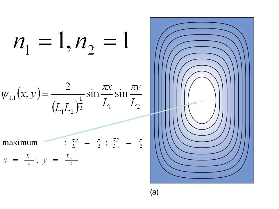
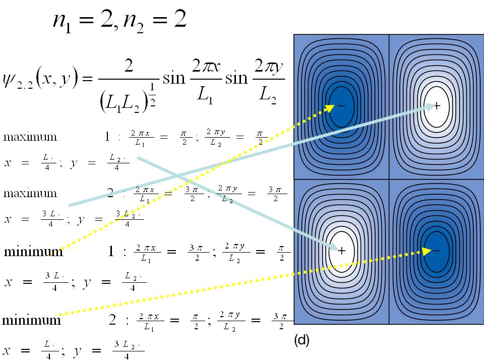
99. Eigenfunctions of a particle on a surface

100. Some wavefunctions of a particle on a surface

105. Picture of the Interactions in an Atom

106. Hamiltonian of Hydrogenic Atoms Only one term Only two terms

107. Magic! 玩個小魔術 Reduced mass

108. How a two-body problem is turned into a one-body problem Center of mass

109. Classical Treatment Free motion of the center of mass One-body (with reduced mass) in a potential

110. Quantum Treatment

111. Motion of the center of massRelative motion

112. Free particle sucks, let’s forget it! Two-body problem  Free particle (Center of mass) + one-body problem

114. Radial Wave Equation

115. Effective potential energy Very different close to the nucleus but similar far from it Solutions of wavefunction and energy for the two cases are very different close to the nucleus but similar to each other at far distances. S orbitals Non-s orbitals

116. Laguerre Equation and Laguerre Polynomials Normalization factor Laguerre polynomails Bohr radius=0.053 nm Bound state

117. Hydrogenic radial wavefunctions Orbitaln l mlml 1s1 0 2s 2 0 2p 21 3s3 0 3p3 1 3d32

118. The radial wavefunctions of the first few hydrogenic atoms of atomic number Z

119. 1s radial wavefunction

120. 2s radial wavefunction

121. 3s radial wavefunction

122. 2p radial wavefunction

123. 3p radial wavefunction

124. An Illustration Calculate (1) the probability density for a 1s- electron at the nucleus and (2) the probability of finding a 2s-electron in a sphere with the nucleus at the center and radius of 0.053 nm. For a 1s-electron: n=1,l=0,m l =0, the wavefunction is Probability density is At the nucleus, r=0,

125. For a 2s-electron, The probability of finding a 2s-electron inside the sphere is

126. Structure of a Hydrogenic Atom Principal quantum number n determines energy Orbital quantum number l gives the angular momentum Magnetic quantum number m l gives the “z”-component of angular momentum

127. Energy Levels unbound state=free state Ground state Rydburg constant Ionization energy For hydrogen atom, E 1 =13.6 eV

128. Spectroscopic Measurement of Ionization Energy

129. Shells and subshells Principal quantum numbers  shells Orbital quantum numbers  subshells

130. Shells and subshells

131. Atomic Orbitals:General Considerations Appropriate balance between potential and kinetic energy (c) (a): electron tends to escape (b): Electron tends to fall into the nucleus

132. Some typical atomic orbitals

134. Node( 節點 / 節面 )

135. Boundary Surface The probability of finding the electron inside the sphere is 90%

136. Mean radius of hydrogenic atoms For 1s

137. Radial Distribution Functions

139. Most probable radius For 1s, Its maximum:

140. The behavior differences between s, p, d and f orbitals near the nucleus s: has big probability amplitude near the nucleus p: probability amplitude ~r near the nucleus d: probability amplitude ~r near the nucleus 2 f: probability amplitude ~r near the nucleus 3

141. 2p Orbitals Nodal plane

142. 3d Orbitals

144. Where are the nodal planes?

145. Quiz 1. Write the recurrence relation for Legendre, Hermite and Laguerre polynomials, respectively. 2. Write the zeroth order and first order Lagendre and Hermite polynomials. 3. Give the approximate expression of the state of a 3p electron in an atom.