Download presentation
Presentation is loading. Please wait.

1
Electromagnetism Christopher R Prior ASTeC Intense Beams Group
Fellow and Tutor in Mathematics Trinity College, Oxford ASTeC Intense Beams Group Rutherford Appleton Laboratory

2
Contents Review of Maxwell’s equations and Lorentz Force Law
Motion of a charged particle under constant Electromagnetic fields Relativistic transformations of fields Electromagnetic energy conservation Electromagnetic waves Waves in vacuo Waves in conducting medium Waves in a uniform conducting guide Simple example TE01 mode Propagation constant, cut-off frequency Group velocity, phase velocity Illustrations

3
Reading J.D. Jackson: Classical Electrodynamics
H.D. Young and R.A. Freedman: University Physics (with Modern Physics) P.C. Clemmow: Electromagnetic Theory Feynmann Lectures on Physics W.K.H. Panofsky and M.N. Phillips: Classical Electricity and Magnetism G.L. Pollack and D.R. Stump: Electromagnetism
 P.C. Clemmow: Electromagnetic Theory. Feynmann Lectures on Physics. W.K.H. Panofsky and M.N. Phillips: Classical Electricity and Magnetism. G.L. Pollack and D.R. Stump: Electromagnetism.")
4
Basic Equations from Vector Calculus
Gradient is normal to surfaces =constant

5
Divergence or Gauss’ Theorem
Basic Vector Calculus Oriented boundary C Stokes’ Theorem Divergence or Gauss’ Theorem Closed surface S, volume V, outward pointing normal

6
What is Electromagnetism?
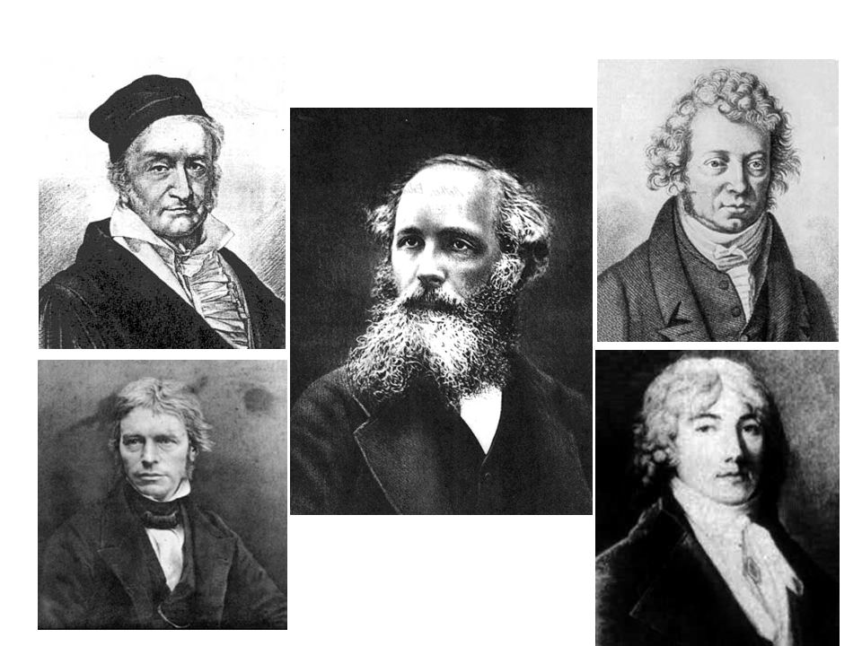
The study of Maxwell’s equations, devised in 1863 to represent the relationships between electric and magnetic fields in the presence of electric charges and currents, whether steady or rapidly fluctuating, in a vacuum or in matter. The equations represent one of the most elegant and concise way to describe the fundamentals of electricity and magnetism. They pull together in a consistent way earlier results known from the work of Gauss, Faraday, Ampère, Biot, Savart and others. Remarkably, Maxwell’s equations are perfectly consistent with the transformations of special relativity.

7
Maxwell’s Equations Relate Electric and Magnetic fields generated by charge and current distributions. E = electric field D = electric displacement H = magnetic field B = magnetic flux density = charge density j = current density 0 (permeability of free space) = 4 10-7 0 (permittivity of free space) = c (speed of light) = m/s 1861 Maxwell had the great idea that unified electricity and magnetism. Made astounding prediction that fleeting electric currents could exist not only in conductors but in all materials, even empty space. Fitted everything together into a single theory. Theory predicted that every time a magnet jiggled or an electric current changed, a wave of energy spread out. He found that waves travelled with speed of light. At a stroke unified electricity, magnetism and light. Astonished everyone, proof took 25 years, when Heinrich Hertz produced waves from a spark-gap source and detected them. Now one of the central pillars of our understanding of the universe, and opened the way to 20th century relativity and quantum theory. Maxwell would have been among the world’s greatest scientists even without his work in electricity and magnetism. His influence is everywhere. He introduced statistical methods into physics; he demonstrated the principle by which we see colours and took the world’s first colour photograph. Maxwell’s demon – molecule-sized creature that could make heat flow from a hot to a cold gas – was the first effective scientific thought experiment. He stimulated the creation of information theory; he wrote a paper on automated control systems that became the foundation of modern control theory and cybernetics. He showed how to use polarised light to reveal strain patterns in a structure; he was the first to suggest a centrifuge to separate gases.
 = 4 0 (permittivity of free space) = c (speed of light) = m/s Maxwell had the great idea that unified electricity and magnetism. Made astounding prediction that fleeting electric currents could exist not only in conductors but in all materials, even empty space. Fitted everything together into a single theory. Theory predicted that every time a magnet jiggled or an electric current changed, a wave of energy spread out. He found that waves travelled with speed of light. At a stroke unified electricity, magnetism and light. Astonished everyone, proof took 25 years, when Heinrich Hertz produced waves from a spark-gap source and detected them. Now one of the central pillars of our understanding of the universe, and opened the way to 20th century relativity and quantum theory. Maxwell would have been among the world’s greatest scientists even without his work in electricity and magnetism. His influence is everywhere. He introduced statistical methods into physics; he demonstrated the principle by which we see colours and took the world’s first colour photograph. Maxwell’s demon – molecule-sized creature that could make heat flow from a hot to a cold gas – was the first effective scientific thought experiment. He stimulated the creation of information theory; he wrote a paper on automated control systems that became the foundation of modern control theory and cybernetics. He showed how to use polarised light to reveal strain patterns in a structure; he was the first to suggest a centrifuge to separate gases.")
8
Maxwell’s 1st Equation Equivalent to Gauss’ Flux Theorem:
The flux of electric field out of a closed region is proportional to the total electric charge Q enclosed within the surface. A point charge q generates an electric field Area integral gives a measure of the net charge enclosed; divergence of the electric field gives the density of the sources.

9
Maxwell’s 2nd Equation Gauss’ law for magnetism:
The net magnetic flux out of any closed surface is zero. Surround a magnetic dipole with a closed surface. The magnetic flux directed inward towards the south pole will equal the flux outward from the north pole. If there were a magnetic monopole source, this would give a non-zero integral. Gauss’ law for magnetism is then a statement that There are no magnetic monopoles

10
Maxwell’s 3rd Equation Equivalent to Faraday’s Law of Induction:
(for a fixed circuit C) The electromotive force round a circuit is proportional to the rate of change of flux of magnetic field, through the circuit. N S Michael Faraday ( ). Apprenticed to a London bookbinder. Became fascinated in science by reading books in the shop. After writing to Davy, was given a job as a lab assistant at the Royal Institution. Became a skilled Chemist. In 1823 discovered that chlorine could be liquefied, also discovered benzene. Discovered e/m induction in His work laid the foundations of all subsequent e/m, leading to devices such as the transformer and electric motor. Was one of the greatest scientific lecturers of the age. Often said to be the greatest experimentalist in the history of science. Faraday’s Law is the basis for electric generators. It also forms the basis for inductors and transformers.
 The electromotive force round a circuit is proportional to the rate of change of flux of magnetic field, through the circuit. N. S. Michael Faraday ( ). Apprenticed to a London bookbinder. Became fascinated in science by reading books in the shop. After writing to Davy, was given a job as a lab assistant at the Royal Institution. Became a skilled Chemist. In 1823 discovered that chlorine could be liquefied, also discovered benzene. Discovered e/m induction in His work laid the foundations of all subsequent e/m, leading to devices such as the transformer and electric motor. Was one of the greatest scientific lecturers of the age. Often said to be the greatest experimentalist in the history of science. Faraday’s Law is the basis for electric generators. It also forms the basis for inductors and transformers.")
11
Maxwell’s 4th Equation Originates from Ampère’s (Circuital) Law :
Satisfied by the field for a steady line current (Biot-Savart Law, 1820): Ampère Biot Andre Marie Ampere ( ), son of a wealthy family from Lyon in France. Did not attend formal school, but was taught at home, mainly by his father. Claimed to have mastered all known mathematics by the age of 12. Submitted first paper at age of 13 (as he was unaware of calculus, this was not thought worthy of publication). Family was badly hit by French revolution (sister died, father guillotined). Became Prof. of Physics and Chemistry at Bourg Ecole Centrale in Published treatises on Mathematical Theory of Games and Calculus of Variations (1803). Appointed tutor at Ecole Polytechnique in Paris in Professor in 1809, chair at Universite de France in Disastrous marriage 1806, separated Worked on partial differential equations, chemistry (fluorine, classification of elements); theory of light (refraction, advocate of wave theory) and a combined theory of electricity and magnetism, produced very quickly after hearing of the Danish physicist Orsted’s experimental work. Discovered electrodynamical forces between linear wires. Similar work also done by Biot and Savart, and by Poisson. Ampere’s most important publication, Memoir on the Mathematical Theory of Electrodynamic Phenomena, was published in 1826, and his theories became fundamental for 19th century developments in electricity and magnetism. Also discovered induction 9 years before Faraday but let the latter have full credit. Ampere’s son achieved fame as a historian, his daughter married one of Napoleon’s lieutenants, who became an alcoholic and the marriage disintegrated acrimoniously. Biot: , Paris.Education at Louis-Le-Grand, followed by the army. Took part in insurrection against government, captured but released after pleadings by Monge. Professor of Mathematics at Beauvais, then at College de France (thanks to Laplace) Professor of Astronomy in Spain. Made advances in astronomy, elasticity, electricity and magnetism, heat and optics; mathematical work in geometry. Together with Savart, discovered that intensity of magnetic field set up by a current in a wire varies inversely with the distance from the wire. Awarded the Rumford Medal of the Royal Society for his work on the polarisation of light passing through chemical solutions.
: Ampère. Biot. Andre Marie Ampere ( ), son of a wealthy family from Lyon in France. Did not attend formal school, but was taught at home, mainly by his father. Claimed to have mastered all known mathematics by the age of 12. Submitted first paper at age of 13 (as he was unaware of calculus, this was not thought worthy of publication). Family was badly hit by French revolution (sister died, father guillotined). Became Prof. of Physics and Chemistry at Bourg Ecole Centrale in Published treatises on Mathematical Theory of Games and Calculus of Variations (1803). Appointed tutor at Ecole Polytechnique in Paris in Professor in 1809, chair at Universite de France in Disastrous marriage 1806, separated Worked on partial differential equations, chemistry (fluorine, classification of elements); theory of light (refraction, advocate of wave theory) and a combined theory of electricity and magnetism, produced very quickly after hearing of the Danish physicist Orsted’s experimental work. Discovered electrodynamical forces between linear wires. Similar work also done by Biot and Savart, and by Poisson. Ampere’s most important publication, Memoir on the Mathematical Theory of Electrodynamic Phenomena, was published in 1826, and his theories became fundamental for 19th century developments in electricity and magnetism. Also discovered induction 9 years before Faraday but let the latter have full credit. Ampere’s son achieved fame as a historian, his daughter married one of Napoleon’s lieutenants, who became an alcoholic and the marriage disintegrated acrimoniously. Biot: , Paris.Education at Louis-Le-Grand, followed by the army. Took part in insurrection against government, captured but released after pleadings by Monge. Professor of Mathematics at Beauvais, then at College de France (thanks to Laplace) Professor of Astronomy in Spain. Made advances in astronomy, elasticity, electricity and magnetism, heat and optics; mathematical work in geometry. Together with Savart, discovered that intensity of magnetic field set up by a current in a wire varies inversely with the distance from the wire. Awarded the Rumford Medal of the Royal Society for his work on the polarisation of light passing through chemical solutions.")
12
Need for Displacement Current
Faraday: vary B-field, generate E-field Maxwell: varying E-field should then produce a B-field, but not covered by Ampère’s Law. Apply Ampère to surface 1 (flat disk): line integral of B = 0I Applied to surface 2, line integral is zero since no current penetrates the deformed surface. In capacitor, , so Displacement current density is Surface 1 Surface 2 Closed loop Current I
: line integral of B = 0I. Applied to surface 2, line integral is zero since no current penetrates the deformed surface. In capacitor, , so. Displacement current density is. Surface 1. Surface 2. Closed loop. Current I.")
13
Consistency with Charge Conservation
Total current flowing out of a region equals the rate of decrease of charge within the volume. From Maxwell’s equations: Take divergence of (modified) Ampère’s equation Charge conservation is implicit in Maxwell’s Equations
 Ampère’s equation. Charge conservation is implicit in Maxwell’s Equations.")
14
Maxwell’s Equations in Vacuum
Source-free equations: Source equations Equivalent integral forms (useful for simple geometries)
")
15
Example: Calculate E from B
z Also from then gives current density necessary to sustain the fields

16
Lorentz Force Law Supplement to Maxwell’s equations, gives force on a charged particle moving in an electromagnetic field: For continuous distributions, have a force density Relativistic equation of motion 4-vector form: 3-vector component:

17
Motion of charged particles in constant magnetic fields
Dot product with v: No acceleration with a magnetic field Dot product with B:

18
Motion in constant magnetic field
Constant magnetic field gives uniform spiral about B with constant energy.

19
Motion in constant Electric Field
Solution of is Energy gain is Constant E-field gives uniform acceleration in straight line

20
Relativistic Transformations of E and B
According to observer O in frame F, particle has velocity v, fields are E and B and Lorentz force is In Frame F, particle is at rest and force is Assume measurements give same charge and force, so Point charge q at rest in F: See a current in F, giving a field Suggests Exact: Rough idea

21
Potentials Magnetic vector potential: Electric scalar potential:
Lorentz Gauge: Use freedom to set

22
Electromagnetic 4-Vectors
Lorentz Gauge 4-gradient 4 4-potential A Current 4-vector Continuity equation Charge-current transformations

23
Relativistic Transformations
4-potential vector: Lorentz transformation Fields:

24
Example: Electromagnetic Field of a Single Particle
Charged particle moving along x-axis of Frame F P has In F, fields are only electrostatic (B=0), given by z b charge q x Frame F v Frame F’ z’ x’ Observer P Origins coincide at t=t=0
, given by. z. b. charge q. x. Frame F. v. Frame F’ z’ x’ Observer P. Origins coincide at t=t=0.")
25
Transform to laboratory frame F:
At non-relativistic energies, ≈ 1, restoring the Biot-Savart law:

26
Electromagnetic Energy
Rate of doing work on unit volume of a system is Substitute for j from Maxwell’s equations and re-arrange into the form Poynting vector

27
Integrated over a volume, have energy conservation law: rate of doing work on system equals rate of increase of stored electromagnetic energy+ rate of energy flow across boundary. electric + magnetic energy densities of the fields Poynting vector gives flux of e/m energy across boundaries

28
Review of Waves 1D wave equation is with general solution
Simple plane wave: Wavelength is Frequency is

29
Phase and group velocities
Superposition of plane waves. While shape is relatively undistorted, pulse travels with the group velocity Plane wave has constant phase at peaks

30
Wave packet structure Phase velocities of individual plane waves making up the wave packet are different, The wave packet will then disperse with time

31
Electromagnetic waves
Maxwell’s equations predict the existence of electromagnetic waves, later discovered by Hertz. No charges, no currents:

32
Nature of Electromagnetic Waves
A general plane wave with angular frequency travelling in the direction of the wave vector k has the form Phase = 2 number of waves and so is a Lorentz invariant. Apply Maxwell’s equations Waves are transverse to the direction of propagation, and and are mutually perpendicular

33
Plane Electromagnetic Wave

34
Plane Electromagnetic Waves
Reminder: The fact that is an invariant tells us that is a Lorentz 4-vector, the 4-Frequency vector. Deduce frequency transforms as

35
Waves in a Conducting Medium
(Ohm’s Law) For a medium of conductivity , Modified Maxwell: Put conduction current displacement current Dissipation factor
 For a medium of conductivity , Modified Maxwell: Put. conduction current. displacement current. Dissipation factor.")
36
Attenuation in a Good Conductor
For a good conductor D >> 1, copper.mov water.mov

37
Charge Density in a Conducting Material
Inside a conductor (Ohm’s law) Continuity equation is Solution is So charge density decays exponentially with time. For a very good conductor, charges flow instantly to the surface to form a surface charge density and (for time varying fields) a surface current. Inside a perfect conductor () E=H=0
 Continuity equation is. Solution is. So charge density decays exponentially with time. For a very good conductor, charges flow instantly to the surface to form a surface charge density and (for time varying fields) a surface current. Inside a perfect conductor () E=H=0.")
38
Maxwell’s Equations in a Uniform Perfectly Conducting Guide
Hollow metallic cylinder with perfectly conducting boundary surfaces z y x Maxwell’s equations with time dependence exp(iwt) are: Assume Then g is the propagation constant Can solve for the fields completely in terms of Ez and Hz
 are: Assume. Then. g is the propagation constant. Can solve for the fields completely in terms of Ez and Hz.")
39
Special cases Transverse magnetic (TM modes):
Hz=0 everywhere, Ez=0 on cylindrical boundary Transverse electric (TE modes): Ez=0 everywhere, on cylindrical boundary Transverse electromagnetic (TEM modes): Ez=Hz=0 everywhere requires
: Ez=0 everywhere, on cylindrical boundary. Transverse electromagnetic (TEM modes): Ez=Hz=0 everywhere. requires.")
40
A simple model: “Parallel Plate Waveguide”
Transport between two infinite conducting plates (TE01 mode): z x y x=0 x=a To satisfy boundary conditions, E=0 on x=0 and x=a, so Propagation constant is
: z. x. y. x=0. x=a. To satisfy boundary conditions, E=0 on x=0 and x=a, so. Propagation constant is.")
41
For given frequency, convenient to choose a s.t. only n=1 mode occurs.
Cut-off frequency, wc w<wc gives real solution for g, so attenuation only. No wave propagates: cut-off modes. w>wc gives purely imaginary solution for g, and a wave propagates without attenuation. For a given frequency w only a finite number of modes can propagate. For given frequency, convenient to choose a s.t. only n=1 mode occurs.

42
Propagated Electromagnetic Fields
From z x

43
Phase and group velocities in the simple wave guide
Wave number: Wavelength: Phase velocity: Group velocity:

44
Calculation of Wave Properties
If a=3 cm, cut-off frequency of lowest order mode is At 7 GHz, only the n=1 mode propagates and

45
Waveguide animations TE1 mode above cut-off ppwg_1-1.mov
TE1 mode, smaller ppwg_1-2.mov TE1 mode at cut-off ppwg_1-3.mov TE1 mode below cut-off ppwg_1-4.mov TE1 mode, variable ppwg_1_vf.mov TE2 mode above cut-off ppwg_2-1.mov TE2 mode, smaller ppwg_2-2.mov TE2 mode at cut-off ppwg_2-3.mov TE2 mode below cut-off ppwg_2-4.mov

46
Flow of EM energy along the simple guide
Fields (w>wc) are: Total e/m energy density Time-averaged energy:
 are: Total e/m energy density. Time-averaged energy:")
47
Poynting Vector Poynting vector is Time-averaged: Integrate over x:
Total e/m energy density Integrate over x: So energy is transported at a rate: Electromagnetic energy is transported down the waveguide with the group velocity

Similar presentations


.>")


.>")


x x f(x x z y. Physics 1304: Lecture 17, Pg 2 Lecture Outline l Electromagnetic Waves: Experimental l Ampere’s Law Is.>")


