Download presentation
Presentation is loading. Please wait.

1
MATLAB INTRO CONTROL LAB1 The Environment The command prompt Getting Help : e.g help sin, lookfor cos Variables Vectors, Matrices, and Linear Algebra (det, inv …) Plotting, plot(x,y,’r’), hist (colormap([0 0 0])), semilog, loglog
![MATLAB INTRO CONTROL LAB1 The Environment The command prompt Getting Help : e.g help sin, lookfor cos Variables Vectors, Matrices, and Linear Algebra (det, inv …) Plotting, plot(x,y,’r’), hist (colormap([0 0 0])), semilog, loglog](http://images.slideplayer.com/23/6640603/slides/slide_1.jpg "MATLAB INTRO CONTROL LAB1 The Environment The command prompt Getting Help : e.g help sin, lookfor cos Variables Vectors, Matrices, and Linear Algebra (det, inv …) Plotting, plot(x,y,’r’), hist (colormap([0 0 0])), semilog, loglog")
2
GETTING HELP type one of following commands in the command window: help – lists all the help topic help topic – provides help for the specified topic help command – provides help for the specified command help help – provides information on use of the help command helpwin – opens a separate help window for navigation lookfor keyword – Search all M-files for keyword

3
VARIABLES Variable names: Must start with a letter May contain only letters, digits, and the underscore “_” Matlab is case sensitive, i.e. one & OnE are different variables. Matlab only recognizes the first 31 characters in a variable name. Assignment statement: Variable = number; Variable = expression; Example: >> tutorial = 1234; >> tutorial = 1234 tutorial = 1234 NOTE: when a semi-colon ”;” is placed at the end of each command, the result is not displayed

4
VARIABLE CONT(‘) Special variables: ans : default variable name for the result pi: = 3.1415926………… eps: = 2.2204e-016, smallest amount by which 2 numbers can differ. Inf or inf : , infinity NaN or nan: not-a-number Commands involving variables: who: lists the names of defined variables whos: lists the names and sizes of defined variables clear: clears all varialbes, reset the default values of special variables. clear name: clears the variable name clc: clears the command window clf: clears the current figure and the graph window.

5
A row vector in MATLAB can be created by an explicit list, starting with a left bracket, entering the values separated by spaces (or commas) and closing the vector with a righ bracket. A column vector can be created the same way, and the rows are separated by semicolo VECTORS,MATRIXES,ARRAYS LINEAR ALGEBRA Example: >> x = [ 0 0.25*pi 0.5*pi 0.75*pi pi ] x = 0 0.7854 1.5708 2.3562 3.1416 x is a row vector. >> y = [ 0; 0.25*pi; 0.5*pi; 0.75*pi; pi ] y = 0 0.7854 1.5708 2.3562 3.1416 y is a column vector.

6
VECTORS CONT’ Vector Addressing – A vector element is addressed in MATLAB with index enclosed in parentheses. Example: >> x(3) ans = 1.5708 1st to 3rd elements of vector x The colon notation may be used to address a block of elements. (start : increment : end) start is the starting index, increment is the amount to add to each successive is the ending index. A shortened format (start : end) may be used if increment Example: >> x(1:3) ans = 0 0.7854 1.5708 3rd element of vector x
 ans = 1st to 3rd elements of vector x The colon notation may be used to address a block of elements. (start : increment : end) start is the starting index, increment is the amount to add to each successive is the ending index. A shortened format (start : end) may be used if increment Example: >> x(1:3) ans = 3rd element of vector x.")
7
MATRIX A is an m x n matrix. A Matrix array is two-dimensional, having both multiple rows and multiple co similar to vector arrays: it begins with [, and end with ] spaces or commas are used to separate elements in a row semicolon or enter is used to separate rows. Example: >> f = [ 1 2 3; 4 5 6 f = 1 2 3 4 5 6 >> h = [ 2 4 6 1 3 5] h = 2 4 6 1 3 5

8
MATRIX CONT Matrix Addressing: -- matrixname(row, column) -- colon may be used in place of a row or column referrs the entire row or column. recall: f = 1 2 3 4 5 h = 2 4 6 1 3 5 Example: >> f(2,3) ans = 6 >> h(:,1) ans = 2 1
 ans = 6 >> h(:,1) ans = 2 1.")
9
SOME USEFUL COMMANDS: zeros(n) returns a n x n matrix of zeroes zeros (m,n) returns a m x n matrix of zeroes ones(n) returns a n x n matrix of ones ones(m,n) returns a m x n matrix of ones rand(n) returns a n x n matrix of random number rand(m,n) returns a m x n matrix of random number size (A) for a m x n matrix A, returns the row vector [m,n] containing the number of rows and columns in matrix. length(A) returns the larger of the number of rows or columns in A
![SOME USEFUL COMMANDS: zeros(n) returns a n x n matrix of zeroes zeros (m,n) returns a m x n matrix of zeroes ones(n) returns a n x n matrix of ones ones(m,n) returns a m x n matrix of ones rand(n) returns a n x n matrix of random number rand(m,n) returns a m x n matrix of random number size (A) for a m x n matrix A, returns the row vector [m,n] containing the number of rows and columns in matrix.](http://images.slideplayer.com/23/6640603/slides/slide_9.jpg " length(A) returns the larger of the number of rows or columns in A.")
11
Scalar-Array Mathematics For addition, subtraction, multiplication, and division of an array by a scalar simply apply the operations to all elements of the array. Example: >> f = [ 1 2; 3 4] f = 1 2 3 4 >> g = 2*f – 1 Each element in the g = multiplied by 2, then subtracted 1 3 by 1. 5 7

12
Example: >> x = [ 1 2 3 ]; >> y = [ 4 5 6 ]; >> z = x.* y z = 4 10 18
![Example: >> x = [ ]; >> y = [ ]; >> z = x.* y z =](http://images.slideplayer.com/23/6640603/slides/slide_12.jpg "Example: >> x = [ ]; >> y = [ ]; >> z = x.* y z =")
14
Solution by Matrix Inverse: Ax = b A-1 Ax = A-1 b x = A-1 b MATLAB: >> A = [ 3 2 -1; -1 3 2; 1 -1 -1]; >> b = [ 10; 5; -1]; >> x = inv(A)*b x = -2.0000 5.0000 -6.0000 Answer: x 1 = -2, x2 = 5, x3 = -6 Solution by Matrix Division: The solution to the equation Ax = b can be computed using left division. MATLAB: Answer: >> A = [ 3 2 -1; -1 3 2; 1 -1 -1]; >> b = [ 10; 5; -1]; >> x = A\b x = -2.0000 5.0000 -6.0000 x1 = -2, x2 = 5, x3 = -6
![Solution by Matrix Inverse: Ax = b A-1 Ax = A-1 b x = A-1 b MATLAB: >> A = [ ; ; ]; >> b = [ 10; 5; -1]; >> x = inv(A)*b x = Answer: x 1 = -2, x2 = 5, x3 = -6 Solution by Matrix Division: The solution to the equation Ax = b can be computed using left division.](http://images.slideplayer.com/23/6640603/slides/slide_14.jpg "MATLAB: Answer: >> A = [ ; ; ]; >> b = [ 10; 5; -1]; >> x = A\b x = x1 = -2, x2 = 5, x3 = -6.")
15
Plotting Curves: plot (x,y) – generates a linear plot of the values of x (horizontal axis) and y (vertical axis). semilogx (x,y) – generate a plot of the values of x and y using a logarithmic scale for x and a linear scale for y. semilogy (x,y) – generate a plot of the values of x and y using a linear scale for x and a logarithmic scale for y. loglog(x,y) – generate a plot of the values of x and y using logarithmic scales for both x and y.
 – generate a plot of the values of x and y using a logarithmic scale for x and a linear scale for y. semilogy (x,y) – generate a plot of the values of x and y using a linear scale for x and a logarithmic scale for y. loglog(x,y) – generate a plot of the values of x and y using logarithmic scales for both x and y..")
16
Multiple Curves: plot (x, y, w, z) – multiple curves can be plotted on the same graph by using multiple arguments in a plot command. The variables x, y, w, and z are vectors. Two curves will be plotted: y vs. x, and z vs. w. legend (‘string1’, ‘string2’,…) – used to distinguish between plots on the same graph Multiple Figures: figure (n) – used in creation of multiple plot windows. place this command before the plot() command, and the corresponding figure will be labeled as “Figure n” close – closes the figure n window. close all – closes all the figure windows. Subplots: subplot (m, n, p) – m by n grid of windows, with p specifying the current plot as the pth window
 – used to distinguish between plots on the same graph Multiple Figures: figure (n) – used in creation of multiple plot windows. place this command before the plot() command, and the corresponding figure will be labeled as Figure n close – closes the figure n window. close all – closes all the figure windows. Subplots: subplot (m, n, p) – m by n grid of windows, with p specifying the current plot as the pth window.")
17
Example: (polynomial function) plot the polynomial using linear/linear scale, log/ linear scale, linear/log scale, & log/log scale: y = 2x^2 + 7x + 9 CODE % Generate the polynomial: x = linspace (0, 10, 100); y = 2*x.^2 + 7*x + 9; % plotting the polynomial: figure (1); subplot (2,2,1), plot (x,y); title ('Polynomial, linear/linear scale'); ylabel ('y'), grid; subplot (2,2,2), semilogx (x,y); title ('Polynomial, log/linear scale'); ylabel ('y'), grid; subplot (2,2,3), semilogy (x,y); title ('Polynomial, linear/log scale'); xlabel('x'), ylabel ('y'), grid; subplot (2,2,4), loglog (x,y); title ('Polynomial, log/log scale'); xlabel('x'), ylabel ('y'), grid;
 plot the polynomial using linear/linear scale, log/ linear scale, linear/log scale, & log/log scale: y = 2x^2 + 7x + 9 CODE % Generate the polynomial: x = linspace (0, 10, 100); y = 2*x.^2 + 7*x + 9; % plotting the polynomial: figure (1); subplot (2,2,1), plot (x,y); title ( Polynomial, linear/linear scale ); ylabel ( y ), grid; subplot (2,2,2), semilogx (x,y); title ( Polynomial, log/linear scale ); ylabel ( y ), grid; subplot (2,2,3), semilogy (x,y); title ( Polynomial, linear/log scale ); xlabel( x ), ylabel ( y ), grid; subplot (2,2,4), loglog (x,y); title ( Polynomial, log/log scale ); xlabel( x ), ylabel ( y ), grid;")
18
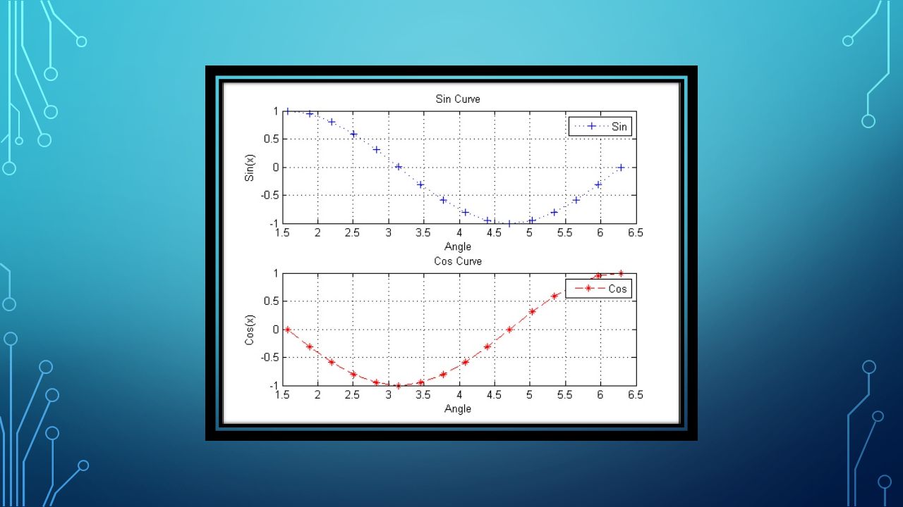
Exercise 1: Use Matlab command to obtain the following a) Extract the fourth row of the matrix generated by magic(6) b) Show the results of ‘x’ multiply by ‘y’ and ‘y’ divides by ‘x’. Given x = [0:0.1:1.1] and y = [10:21] c) Generate random matrix ‘r’ of size 4 by 5 with number varying between -8 and 9 Exercise 2: Use MATLAB commands to get exactly as the figure shown below x=pi/2:pi/10:2*pi; y=sin(x); z=cos(x);
 Generate random matrix ‘r’ of size 4 by 5 with number varying between -8 and 9 Exercise 2: Use MATLAB commands to get exactly as the figure shown below x=pi/2:pi/10:2*pi; y=sin(x); z=cos(x);.")
Similar presentations


, Arithmetical Operations, Defining and manipulating.>")


 where all variables reside After carrying out a calculation, MATLAB assigns the result.>")


