1. Chapters 5 and 6: Numerical Integration

2. Definition of Integral by
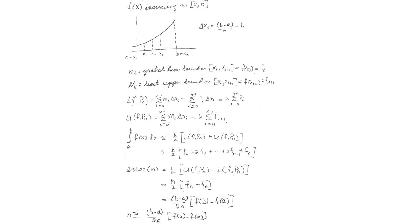
Upper and Lower Sums
n=number of partitions

3. Application to monotone decreasing function
Divide [a,b] into n subintervals using n+1 equally spaced points
h=(b-a)/n is subinterval width

4. “composite trapezoid rule”

5. How would this change for monotone increasing function?
Divide [a,b] into n subintervals using n+1 equally spaced points
h=(b-a)/n is subinterval width
How would this change for
monotone increasing function?

6. How would this change for monotone increasing function?
“composite trapezoid rule”
How would this change for
monotone increasing function?

8. Derive the trapezoid rule for any f(x)

9. Replace f(x) on [a,b] by line p(x)
Area under p(x) on [a,b] is a trapezoid = (b-a)(f(a)+f(b))/2
Pseudo code for trapezoid rule with arbitrarily spaced points
Trap_Arbitrary_Points(x,f)
n=length(x);
sum=0;
for i=2 to n
sum=sum+(xk – xk-1)(fk + fk-1)/2;
Usually x1 = a and xn = b

10. Pseudo code for trapezoid rule with arbitrarily spaced points
Trap_Arbitrary_Points(x,f)
n=length(x);
sum=0;
for i=2 to n
sum=sum+(xk – xk-1)(fk + fk-1)/2;
Write MatLab code for Trap_Arbitrairy_Points(x,f)
Test on
with 10 logarithmically spaced points between 1 and 5

11. Replace f(x) on [a,b] by line p(x)
“composite” trapezoid rule is a special case of Trap-Arbitrary-Points
Samples of the integrand are equally spaced in the range of integration
Pseudo code for composite trapezoid rule
Composite_Trap_Rule(fh,a,b,npts)
x=linspace(a,b,npts);
call Trap_Arbitrary_Points(x,fh(x));

12. Pseudo code for composite trapezoid rule
Composite_Trap_Rule(fh,a,b,npts)
x=linspace(a,b,npts);
call Trap_Arbitrary_Points(x,fh(x))
Write MatLab code for Composite_Trap_Rule(fh,a,b,npts)
Test on
with 10 equally spaced points between 1 and 5

13. For given number of points, accuracy of numerical integration
depends on where the integrand is evaluated
Accuracy of numerical integration also depends on the
variable of integration
Consider
approximated by the trapezoid rule with
(a) equally spaced points in the interval 1<x<5
(b) logarithmically spaced points in the interval 1<x<5
(c) equally spaced points with integration variable
y = ln(x)

14. Changing variable of integration

15. Use the transformation y = ln(x) to change the variable of integration
Use the transformation y = ln(x) to change the variable of integration. dy = dx/x
x(y)= exp(y)
Integrand is a function of y through x(y)

16. Compare 3 ways to evaluate

17. Replacing f(x) by polynomial p(x) is a
common numerical integration strategy
Area under p(x) on [a,b] is integral of the polynomial between a and b,
which can be done analytically if we know the coefficients.
Given values of the integrand f(x) at n points we can determine a
polynomial of degree n-1 that passes through those points.
If we are given only f(a) and f(b) we can determine the equation of a
line (degree=1) that passes through them.

18. Which is the same result that we got using the area of trapezoid

19. Replace f(x) on [a,b] by line p(x)
Pseudo code for composite trapezoid rule without call to Trap_Arbitrary_Points
CTR(fh,a,b,npts)
h=(b-a)/(npts-1)
CTR=(fh(a)+fh(b))h/2
if npts > 2
CTR=CTR+h(sum of “internal” samples of integrand)
Every numerical integration formula has the form:
(range of integration) (average of integrand on that range)

20. Use Taylor formula to derive an expression for the
expected error in the trapezoid rule for any function
with a continuous second derivative

21. Error in Trap Rule: single subinterval of size h
Taylor-series expression for exact result

22. Error in Trap Rule: single subinterval of size h
From previous slide
Difference between exact
and trapezoid rule

23. Error in Trap Rule: n subinterval of size h1
n is number of subinterval
Equals number of points -1

24. For the trapezoid rule
Error estimate e = (b – a)3|f ‘’(x)|/12n2 applies to any
continuous integrand f(x) on [a,b]
Error estimate e = (b – a)[f(b) - f(a)]/2n applies to any
monotone increasing integrand f(x) on [a,b]
Error estimate e = (b – a)[f(a) - f(b)]/2n applies to any
monotone decreasing integrand f(x) on [a,b]
Exact error can evaluated when the anti-derivative
of the integrand f(x) is known

25. Assignment 2, Due 2/5/15
Use the error formulas derived in class for the composite trapezoid rule applied to the integral
to obtain 2 estimates of the number of sub-intervals needed to have an error less than 10-4
Write a MabLab function for the composite trapezoid rule with function handle and number of subintervals as parameters. Use this code to discover which of the error estimates is more realistic.

26. Log10(|traprule-exact|)

27. Problems from text on application of error formulas

28. Problem text p 188
Integrand is monotone decreasing. Estimate the number
of points needed for accuracy 0.5x10-4 using the error
formula derived from upper and lower sums.

29. Problem text p 188
n > (b-a) [f(a)-f(b)]/2e
n > (5-2) [1/log10(2)-1/log10(5)]/(1x10-4 ) = 56,738

30. Problem text p 200
Estimate the error if the integral
is evaluated by the composite trapezoid rule with 3 points
|error| < (b-a)3|f’’(x)|max /12n2
Plot |f’’(x)| to estimate maximum value on [0, 1]

31. f ``(x) = (6x2 -2)/(x2 +1)3
|f’’(x)| X

32. Problem text p 200
Estimate the error if the integral
is evaluated by the composite trapezoid rule with 3 points
|error| < (b-a)3|f’’(x)|max /12n2 = (1)(2)/((12)(9)) = 1/54
Correct answer is 1/24. What is wrong?

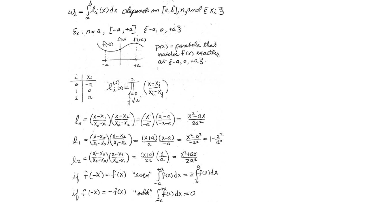
33. Most numerical integration formulas have the form
Example: Trapezoid rule
w0 = wn = 1/2n
wk = 1/n if 1< k<n-1
n = number of intervals
One approach to deriving such formulas:
Replace the integrand by the Lagrange
interpolation formula

34. p(x) “Lagrange interpolation formula” is a polynomial of degree n
that passes through a set of n+1 user-supplied point {xk,f(xk)}.
p(x)
Regardless of where {xk} are in [a,b], this integration formula
will be exact for polynomials of degree up to n. Usually {xk}
are chosen to make the formula exact for higher-degree
polynomials.

36. Simpson’s rule for one pair of subintervals

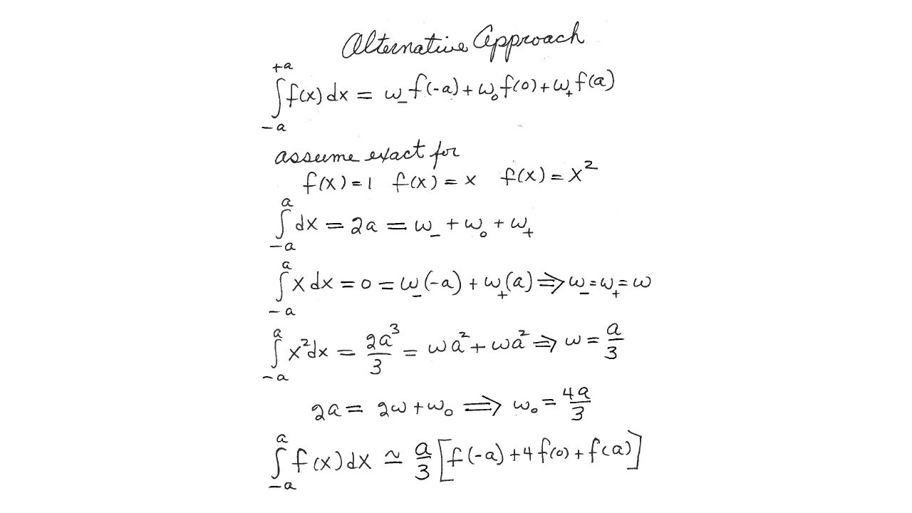
37. Same result by simpler approach

39. n pairs of subintervals

40. Problem text p228
Evaluated by composite Simpson’s rule with 5 points
Bound the error
|error| = (b-a)h4|f(4)(x)|/180 a < x < b (text p221)
h = width subintervals
Since |error| proportional to |f(4)(x)|, Simpson’s rule is exact for a cubic, one degree higher than we should expect from number of samples of the integrand

41. Problem text p228, 6th ed
Evaluated by composite Simpson’s rule with 5 points
Bound the error
|error| = (b-a)h4|f(4)(x)|/180 a < x < b (text p221)
h = width subintervals
In this case, h = 0.25
f(4)(x) = 24/x5 |f(4)(x)| < 24 1<x<2
|error| = (1)(0.25)4 24/180 =

42. Another example of deriving
integration formulas
Why is this different from
Simpson’s rule?

43. Same example by simpler approach

45. Which is likely to
be more accurate?

46. Problems from text p240 on deriving integration formulas
6.2-5
6.2-6
6.2-9

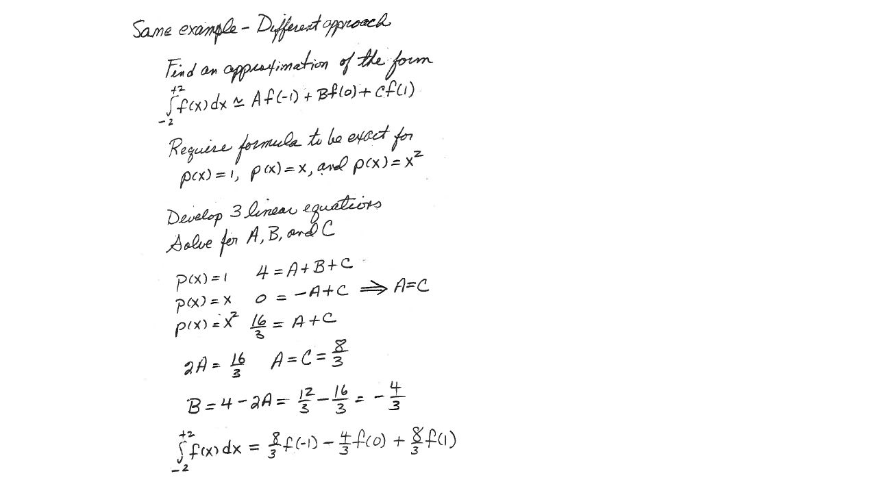
47. Example text p240
Find A and B by requiring formula to be exact for
f(x) = 1 and f(x) = x

48. Example 6.2-6 text p240 f(x) = 1, f `(x) = 0, f(x) = x, f `(x) = 1,
B = (b2 - a2)/2 - Aa = (b2-a2)/2 - (b-a)a

49. Assignment 3, Due 2/12/15:
1. How many samples of the integrand are required to estimate
with error less than by the composite trapezoid rule
and the composite Simpson’s rule. Show all derivation steps
2. Problem p240, 6th edition; exercise p248, 7th
edition. Show all derivation steps.

50. Let {x0, x1, …, xn} be n+1 points on [a, b] where integrand
evaluated.
Will be exact for polynomials of degree n
Trapezoid rule: (n = 1) exact for a line
In general, error proportional to |f’’(z)|
Simpson’s rule: (n = 2) exact for a parabola
In general, error proportional to |f(4)(z)|
How could this happen?

51. 0 < k < n number of nodes = degree of polynomial
Gauss quadrature extents Simpson’s rule idea to its logical
extreme: Give up all freedom about where the integrand will
be evaluated to maximize the degree of polynomial for which
formula is exact.
nodes {x0, x1, …, xn} exist on [a, b] such that
is exact for polynomials of degree at most 2n+1
Nodes are zeros of polynomial g(x) of degree n+1 defined by
0 < k < n number of nodes =
degree of polynomial

52. Proof of Gauss quadrature theorem

53. For any set of n+1 nodes on [a,b]
zeros

54. For any set of n+1 nodes on [a,b],
Summary of Gauss Quadrature Theorem
For any set of n+1 nodes on [a,b],
is exact for polynomials up to degree n
For the special set of node in Gauss quadrature, the formula is
correct of polynomials of degree at most 2n+1
Nodes and weights, Ai, depend on both [a,b] and n
Scaling property of integrals lessens the impact of these dependences

55. Degree of g(x) = number of nodes
Number of conditions on
g(x) = number of nodes
Number of conditions not
Sufficient to determine all
coefficients
Terms with odd powers of x
in g(x) do not contribute
due to symmetry

56. Determines ratio of C1 and C3 only.
As noted before, number of
conditions on g(x) insufficient
to determine all 4 coefficients
of a cubic

57. Using plan (b)

58. Using plan (b)

59. Points and weights of Gauss quadrature are determined for
Every integral from a to b can transformed into integral from -1 to 1

60. Nodes and weights determined
for [-1,1] can be used for [a,b]
Given values of y from table, this x(y)
determines values on [a,b] where
integrand will be evaluated

61. From text p236, 6th edition
Note: n = number of intervals
Example:
note symmetry of points
and weights

62. (no anti-derivative)
with 2 nodes

63. Pseudo-code GQ2345(a,b,f)
% Gauss quadrature for integral of f between a and b with 2-5 points
calculate scale factor and coefficients in x(y)
for each number of points
calculate points and weights by formulas in text
calculate where in [a,b] integrand will be sampled
calculate samples of integrand
calculate weighted average of integrand samples
multiply by scale factor
return values
Including symmetry of points and weights is optional

64. Assignment 4, Due 2/19/15:
Write MATLAB codes for composite Simpson’s rule
and Gauss-quadrature
Make a table that compares the relative error
(percent difference from exact value) in
approximated by the composite trapezoid rule, the
composite Simpson’s rule and Gauss quadrature
when the integrand is evaluated at 2, 3, 4, and 5 points,
if possible.

65. Quiz #4
Deriving integration formulas

66. More extensive tables of nodes and weights than given in text.
Note that symmetry used to compress the table
Verify that values for n = 2 to 5 are the same as n = 1 to 4 in table on
P236 of text

67. Why is the integral
hard to evaluate by numerical integration?
Does the integral have a finite value?
If so, can it be estimated by trapezoid rule,
Simpson’s rule and Gauss quadrature?

68. Change the variable of integration in
by the transformation y = ln(1/x) = -ln(x)

69. By arguments similar to the Guass-quadrature theorem,
Laguerre derived an approximation to infinite integrals
in which the integrand is evaluated at the zeroes of the
Laguerre polynomials
This formula only can be applied when f(x) is rapidly
decreasing with increasing x

70. Note less symmetry than with
Gauss quadrature
Use first and last columns
For n > 6 see me

71. Pseudo-code LQ2345(f)
% Leguerre quadrature for integral of f between 0 and infinity with 2-5 points
for each number of points
enter points and weights from table
calculate integrand where it is to be sampled
calculate weighted average of integrand samples
return values

72. Assignment 5, Due 2/24/15:
Write MATLAB codes to approximate the integral
after the transformation y = ln(1/x) changes it into a form where Laguerre integration can be applied.
Make a graph that compares, as a function of the number of points
where the integrand is evaluated, the relative error of the Laguerre
approximation with results obtained when the integral is
evaluated by Gauss quadrature without a change of variable.

73. Suggested problems from the text on numerical integration
Chapter 5.1
Problems 1, 6
Computer problem 2
Chapter 5.2
Problems 2, 4, 7, 12, 13, 15, 16
Computer problems 2 and 5(by Laguerre and Gauss quadrature)
Chapter 6.1
Problems 2, 4,
Chapter 6.2
Problems 1, 5, 6, 9, 11, 12
Computer problems 2, 3, 6, 8, 10

74. Computer problems 6.2-2 and 6.2-3 p241
Formula (5) p234 is 3-point Gauss quadrature

75. exact=2
quad=
Trap rule 800 =

76. CP 5.1-2
If the integrand cannot be defined in the
command window with an inline statement,
use an m-file. to inform MatLab.

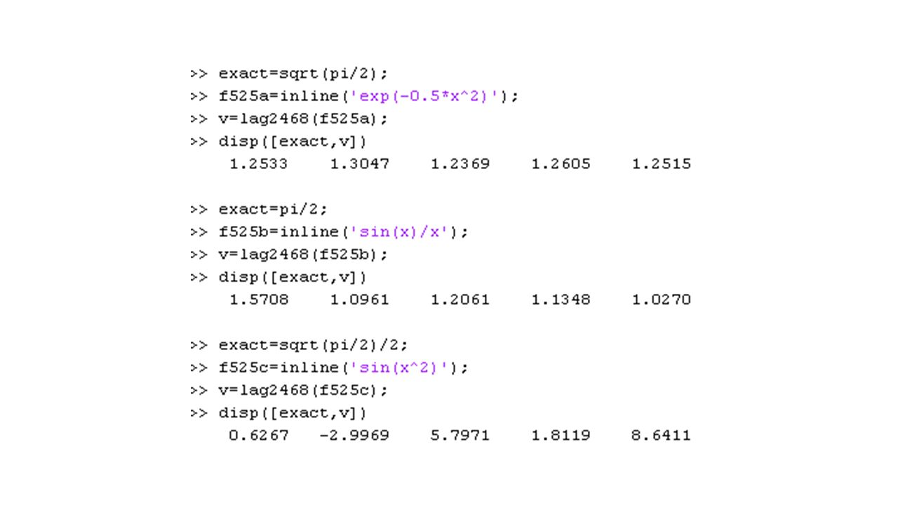
77. Computer problem p203
Approximate by Gauss quadrature

79. = p/2 Computer problem 5.2-5 p204 = sqrt(p/2) = sqrt(p/2)/2
Approximate by Laguerre quadrature

81. = p/2 Computer problem 5.2-5 p204 = sqrt(p/2) = sqrt(p/2)/2
Approximate by Laguerre quadrature

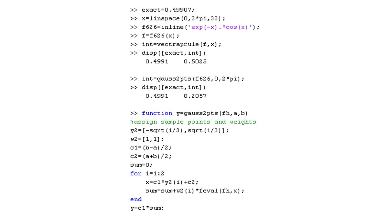
82. Computer problem p242
By 32-point trapezoid rule and 2-point Gauss quadrature

84. Computer problem p242

85. Computer problem 6.2-8 p242 quad=2.0348159 quad=0.4268024
quad with upper limit of 10 =

86. Computer problem p242

87. Computer problem p243