Download presentation
Presentation is loading. Please wait.

2
Chapter 7 Numerical Differentiation and Integration

3
INTRODUCTION DIFFERENTIATION USING DIFFERENCE OPREATORS DIFFERENTIATION USING INTERPOLATION RICHARDSON’S EXTRAPOLATION METHOD NUMERICAL INTEGRATION

4
NEWTON-COTES INTEGRATION FORMULAE
THE TRAPEZOIDAL RULE ( COMPOSITE FORM ) SIMPSON’S RULES ROMBERG’S INTEGRATION DOUBLE INTEGRATION
 SIMPSON’S RULES. ROMBERG’S INTEGRATION. DOUBLE INTEGRATION.")
5
Basic Issues in Integration
What does an integral represent? = AREA = VOLUME

6
NUMERICAL INTEGRATION
Consider the definite integral

8
Then, if n = 2, the integration takes the form

9
Thus Simpson’s 1/3 rule is based on fitting three points with a quadratic.
Similarly, for n = 3, the integration is found to be

11
This is known as Simpson’s 3/8 rule, which is based on fitting four points by a cubic. Still higher order Newton-Cotes integration formulae can be derived for large values of n.

12
TRAPEZOIDAL RULE

14
SIMPSON’S 1/3 RULE

17
Simpson’s 3/8 rule is

18
with the global error E given by

19
ROMBERG’S INTEGRATION
We have observed that the trapezoidal rule of integration of a definite integral is of O(h2), while that of Simpson’s 1/3 and 3/8 rules are of fourth-order accurate.
, while that of Simpson’s 1/3 and 3/8 rules are of fourth-order accurate.")
20
We can improve the accuracy of trapezoidal and Simpson’s rules using Richardson’s extrapolation procedure which is also called Romberg’s integration method.

21
For example, the error in trapezoidal rule of a definite integral

22
can be written in the form

23
By applying Richardson’s extrapolation procedure to trapezoidal rule, we obtain the following general formula

25
where m = 1, 2, … , with IT0 (h) = IT (h). For illustration, we consider the following example.

26
starting with trapezoidal rule, for the tabular values
Example: Using Romberg’s integration method, find the value of starting with trapezoidal rule, for the tabular values

27
x 1.0 1.1 1.2 1.3 1.4 1.5 1.6 1.7 1.8 y = f(x) 1.543 1.669 1.811 1.971 2.151 2.352 2.577 2.828 3.107

28
Solution Taking

29
Let IT denote the integration by Trapezoidal rule, then for

32
Similarly for

33
Now, using Romberg’s formula , we have

35
Thus, after three steps, it is found that the value of the tabulated integral is 1.7671.

36
DOUBLE INTEGRATION To evaluate numerically a double integral of the form

37
over a rectangular region
bounded by the lines x = a, x = b, y = c, y = d we shall employ either trapezoidal rule or Simpson’s rule, repeatedly With respect to one variable at a time.

38
Noting that, both the integrations are just a linear combination of values of the given function at different values of the independent variable, we divide the interval [a, b] into N equal
![Noting that, both the integrations are just a linear combination of values of the given function at different values of the independent variable, we divide the interval [a, b] into N equal](http://slideplayer.com/slide/4619541/15/images/38/Noting+that%2C+both+the+integrations+are+just+a+linear+combination+of+values+of+the+given+function+at+different+values+of+the+independent+variable%2C+we+divide+the+interval+%5Ba%2C+b%5D+into+N+equal.jpg "Noting that, both the integrations are just a linear combination of values of the given function at different values of the independent variable, we divide the interval [a, b] into N equal")
39
sub-intervals of size h, such that h = (b – a)/N; and the interval (c, d) into M equal sub-intervals of size k, so that k = (d – c)/M. Thus, we have

41
Thus, we can generate a table of values of the integrand, and the above procedure of integration is illustrated by considering a couple of examples.

42
Example Evaluate the double integral
by using trapezoidal rule, with h = k = 0.25.

43
Solution Taking x = 1, 1. 25, 1. 50, 1. 75, 2. 0 and y = 1, 1. 25, 1
Solution Taking x = 1, 1.25, 1.50, 1.75, 2.0 and y = 1, 1.25, 1.50, 1.75, 2.0, the following table is generated using the integrand

44
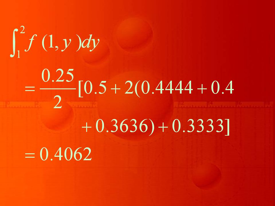
x y 1.00 1.25 1.50 1.75 2.00 0.5 0.4444 0.4 0.3636 0.3333 0.3077 0.2857 0.307 0.2667 0.25

45
Keeping one variable say x fixed and varying the variable y, the application of trapezoidal rule to each row in the above table gives

50
and

51
Therefore,

52
By use of the last equations we get the required result as

53
Example :Evaluate by numerical double integration.

54
Solution Taking x = y = π/4, 3 π /8, π /2, we can generate the following table of the integrand

55
x y π/8 π/4 3π/8 π/2 0.0 0.6186 0.8409 0.9612 1.0

56
Keeping one variable as say x fixed and y as variable, and applying trapezoidal rule to each row of the above table, we get

59
Similarly, we get

60
and

61
Using these results, we finally obtain

Similar presentations


. In order to evaluate definite integral I = a ∫ b y dx = a ∫ b f(x) dx Divide the interval (b-a) of x into n equal.>")


 Section 04 Read Chapter 21, Section 1 Read Chapter.>")


