1. Calculus AB APSI 2015 Day 2 Professional Development Workshop Handbook
Curriculum Framework Calculus AB and BC
Professional Development
Integration, Problem Solving, and Multiple Representations
Curriculum Module

2. Tuesday Morning (Part 1) How f’(a) fails to Exist
Developing Understanding of the Derivative
Upload TI 84 Programs
Big Idea 1: Limits
 Break  
Morning (Part 2)
Ideas That Can Be Explored Before Working with Formulas
Connecting Graphs of f, f’, and f”
Connecting Differentiability with Continuity
Introduction to Local Linearity
How f’(a) fails to Exist
How Can One Graph Help Describe Another Graph?
Lunch
Afternoon (Part 1)
Share an Activity
Discussion of Homework Problems
Break
Afternoon (Part 2)
Slope Fields
Reasoning with Tabular Data
Big Idea 2: - Derivatives

3. Tuesday Assignment - AB
Multiple Choice Questions on the test: 9, 11, 15, 19, 21, 22, 23, 27, 28, 82, 88, 89, 90, 91, 92
Free Response:
2014: AB3, AB6
2015: AB2, AB3/BC3

4. Numerical Approach
Students should explore understanding the forward difference quotient, the backwards difference quotient, and the symmetric difference quotient

5. Forward Difference Quotient

6. Backward Difference Quotient

7. Symmetric Difference Quotient

8. Definition of a Derivative at x=a
All lead to the derivative of a function at a point x=a.
Activities with the graphing calculator can numerically and graphically develop understanding for the algebraic approach.

9. Understanding The Derivative Numerically Using Difference Quotients
Activity

10. Understanding The Derivative Graphically Using Difference Quotients
Activity

11. The values of a derivative are not random
The values of a derivative are not random. They are values of a function defined by As we saw in the first two activities this limit defines a function of x, not a number.

12. Example
Do you see how this relates to the activity we did on the difference quotients?

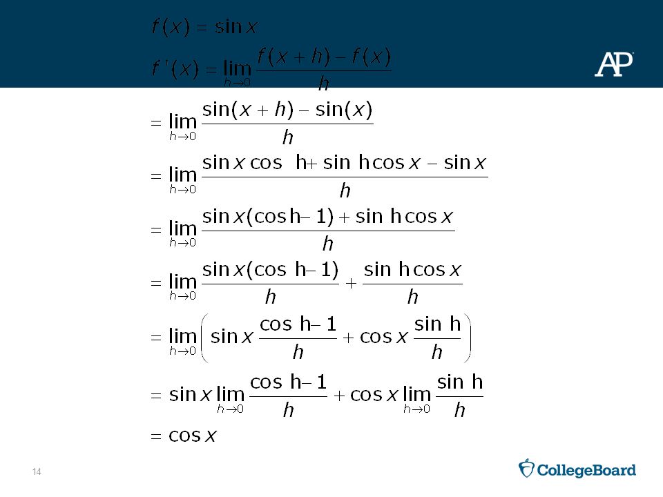
13. Building upon these activities it is now appropriate to explore the analytical approach to the definition of a derivative

15. You may want to go on and learn other properties of the derivative and uses of the derivative before you actually derive the formulas for the derivatives.
Once you get into the formulas that’s where the emphasis will be and not on the concept.

16. Making Observations about the Function and Its Derivative
When y1 is increasing, what do you notice about the values of y2?
When y1 is decreasing, what do you notice about the values of y2?
When y1 reaches a maximum, what do you notice about the value of y2?

17. Making Observations about the Function and Its Derivative
When y2 is equal to zero, what do you notice about the behavior of y1?
Would you describe y1 as concave down or concave up? How would you describe the slope of y2?
Activity

18. Upload TI 84 Programs

19. Big Idea 1 - Limits
Page

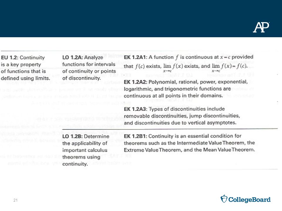
20. Big Idea 1 - Limits

22. Ideas That Can Be Explored Without the Knowing Derivative Formulas
Using any of the difference quotients (with small h values) obtain graphical (and sometimes numerical) information that can be generalized.
The graph of f ’
using the difference
quotient with f
The graph of f “
using the difference
quotient with f ‘
The graph of f

23. Notice that
when the derivative of f is positive the original function f is increasing and tangent lines to f have positive slopes
when the derivative of f is negative the original function f is decreasing and tangent lines to f have negative slopes
when the derivative of f is zero after being positive and then negative the original function f has reached a minimum;
when the derivative of f is zero after being negative and then positive the original function f has reached a maximum. ;
The slope of a tangent line to f at a maximum or minimum is zero.

24. If the derivative of f is positive and decreasing the slope of the original function f must be decreasing (or f is concave down)
If the derivative of f is negative and increasing the slope of the original function f must be increasing or (or f is concave up)
A minimum of f occurs when the derivative of f goes from negative to positive; A maximum of f occurs when the derivative of f goes from positive to negative

25. When the sign changes on the second derivative of f the concavity of f is changing sign and a point of inflection of f has been located
Differentiability of f implies Continuity of f but continuity of f does not imply differentiability of f.

26. Extreme Value Theorem
A function f, continuous on a closed interval, must have both an absolute minimum and maximum value
The location for an extrema is found where the function changes from increasing to decreasing or visa versa
We also need to check the value at either endpoint

27. A derivative of a derivative is the second derivative The 2nd derivative provides the same information about the first derivative that the first derivative provides about the function When the second derivative of a function is positive-the first derivative of the function is increasing –the slope is getting steeper

28. A function f is concave up if f’ is increasing f” is positive or
Concavity
A function f is concave up if
f’ is increasing
f” is positive or
A tangent line to f lies below the graph(except at the point of tangency)

29. A function f is concave down if f’ is decreasing f” is negative or
Concavity
A function f is concave down if
f’ is decreasing
f” is negative or
A tangent line of f lies above the graph(except at the point of tangency)
Concavity is defined on an interval not at a point

30. A Point of Inflection
A point where the second derivative of a function (f”) changes sign (therefore changing the concavity of function f) is called a point of inflection
First find where the second derivative (f”) is zero or undefined. Check on both sides of that point to see if the second derivative (f”) changes sign
Points of inflection correspond to the extreme values of the first derivative (f’) equal zero.

31. The limit only exists from one side
Remember
Functions are not differentiable at the endpoints of a closed interval.
The limit only exists from one side

32. Connecting Graphs of f, f’ and descriptions
Match graphs of f, f ‘ and descriptions of f and f’
Section 3 of Notebook

33. Connecting Continuity and Differentiability
Because a limit is used to define the derivative
If the derivative exists at a point, the function is continuous at that point
Differentiability implies continuity
If a function is differentiable at a point, it is continuous there
If a function is differentiable on an interval, it is continuous on the interval

34. Is a continuous function differentiable
Is a continuous function differentiable? Is a differentiable function continuous?
𝑦1= 𝑥 2 −2
𝑦2= 𝑦1(𝑥+0.001)−𝑦1(𝑥
𝑦1=|𝑥|−2
Activity

35. Local linearity is the graphical approach to the derivative
Local linearity is a property of differentiable functions that says – roughly – that if you zoom in on a point on the graph of the function (with equal scaling horizontally and vertically), the graph will eventually look like a straight line with a slope equal to the derivative of the function at that point.
Local linearity is the graphical approach to the derivative

36. Functions that are differentiable are locally linear, and, conversely, functions that are locally linear are differentiable.
Unfortunately, there is no sure way of determining whether a function is locally linear until you know if it’s differentiable.
Locally linear is a good, informal, way to introduce the concept of the derivative and to let your students see what differentiable means.

37. Local linearity and the secant line approximations can be explored in precalculus without reference to differentiability.
Local linearity can be introduced through zooming out and zooming in
Differentiable functions are smooth Functions that are not differentiable have sharp bends or discontinuities in them

38. Introduction to Local Linearity
Write a rule for each of the three lines. Give justification for why you
wrote each equation. y3 y5
J.T. Sutcliff y1

39. Which line is y1 y3 y5

40. Enter each of these functions in your graphing calculator in a zoom 4 Decimal window. Record your sketch below

41. Zoom in on the origin by resetting the window to [-0. 004, 0. 004, 0
Zoom in on the origin by resetting the window to [-0.004, 0.004, 0.001, , 0.003, 0.001]. What has happened to each of the graphs when you look at a very small window around the origin?

42. We say that a function is locally linear when we can make a curved line appear linear.
Rewrite the equation of each graph at the right now that you know the scale. y2 y4 y6

43. Each straight line equation that you wrote is called a linear approximation for these graphs at the point x = 0.

44. Enter these equations in your graphing and view all six equations in a zoom 4 decimal window.
Compare the six graphs in the zoom in window.

45. Each linear approximation (or equation) is also called a tangent line to the corresponding graph.
Build a table near x = 0and notice how you can approximate y1(.01) by looking at y2(.01).
Also look at y3(.01) and y4(.01) and y5(.01) and y6(.01)

46. Graph the equation in on a zoom 4 decimal window.
Zoom in to a small window and write the equation of the line that can be used as the linear approximation for this function at x = 0.

47. How f’(a) Fails to Exist
Activity

48. Sample Differentiation Lessons
Thinking about the Derivative of a Function
The Rules for Differentiation

49. Monday - AB
Multiple Choice Questions on the 2014 test: 9, 11, 15, 19, 21, 22, 23, 27, 28, 82, 88, 89, 90, 91, 92
Free Response:
2014: AB1, AB2
2015: AB1/BC1, AB6

50. 2014 AB1

51. Scoring Rubric for 2014 AB1

52. Calculus in Motion Animation of 2014 AB1

53. 2014 AB2

54. Scoring Rubric for 2014 AB2

55. 2015 AB1

56. Scoring Rubric 2015 AB1

57. 2015 AB6

58. 2015 AB6 Scoring Rubric

59. There are two different types of problems in an AP Calculus course.
Slope Fields
There are two different types of problems in an AP Calculus course.
In one type, you are given a function and then asked about its rate of change;
in the other type, you are given how the function changes and then asked to identify the function.
Thus derivative and antiderivative permeate the course.

60. The term differential equation may seem formidable at first, but since a differential equation is nothing more than an equation that involves a derivative, differential equations occur throughout the course. A solution to a differential equation is simply a function that satisfies the equation.

61. Introducing the a Slope Field
Most people think that if they are handed a differential equation the task will be to solve it.
But what is a differential equation really describing?
Students can be asked to describe the behavior or tangent lines based on the differential equation.
Introducing Slope Fields (Smartboard)

62. Create a Slope field

63. Creating Basic Slope Fields

64. Using Technology to Create Slope Fields
Reading Slope Fields

65. Nancy Stephenson’s Materials on AP Central
Slope Field Handout
Slope Field Card Match

66. What to include in your study
Build activities so that student
become familiar with the terminology of differential equations
recognize what is meant by a solution to a differential equation
use differential equations in modeling applications
understand the relationship between a slope field and a solution curve for the differential equation

67. What might students be asked to do
verify whether or not a given function is a solution to a differential equation
manually construct a portion of a slope field for a given differential equation
choose from among many differential equations which one is associated with a given slope field

68. Choose from among many slope fields which one is associated with a given differential equation
Recognize exponential growth and decay, the governing differential
equation and its solution
Solve a given separable differential equation

69. Solve a given separable differential equation
is a solution to a differential equation if and only if

70. Slope Field Matching Cards
Section 4 of Notebook

71. Reasoning with Tabular Data
2008 Curriculum Module

72. Instantaneous Rate of Change
Pages 1 and 2
Approximate y’(12) and explain the meaning of y’(12) in terms of the population of the town.

73. Average Value of a Function
Pages 1 and 2
Approximate, with a trapezoidal rule, the average population of the town over the 20 years.

74. Approximate an Integral
Pages 3 and 4
Use a midpoint Riemann sum with three subintervals to approximate
Explain the meaning of this definite integral in terms of the water flow, using correct units.

75. Evaluate an Average Rate
Pages 4 and 5
Use P(t) to find the average rate of water flow during the 12-hour period. Indicate units of measure.

76. Approximate a Total Distance Traveled
Pages 5 and 6
Approximate the distance traveled over
Using a right Riemann sum with four intervals.

77. Use P(t) to find the average rate of water flow during the 12-hour time period. Indicate units of measure.

78. Other AP Free Response questions that reference tabular data

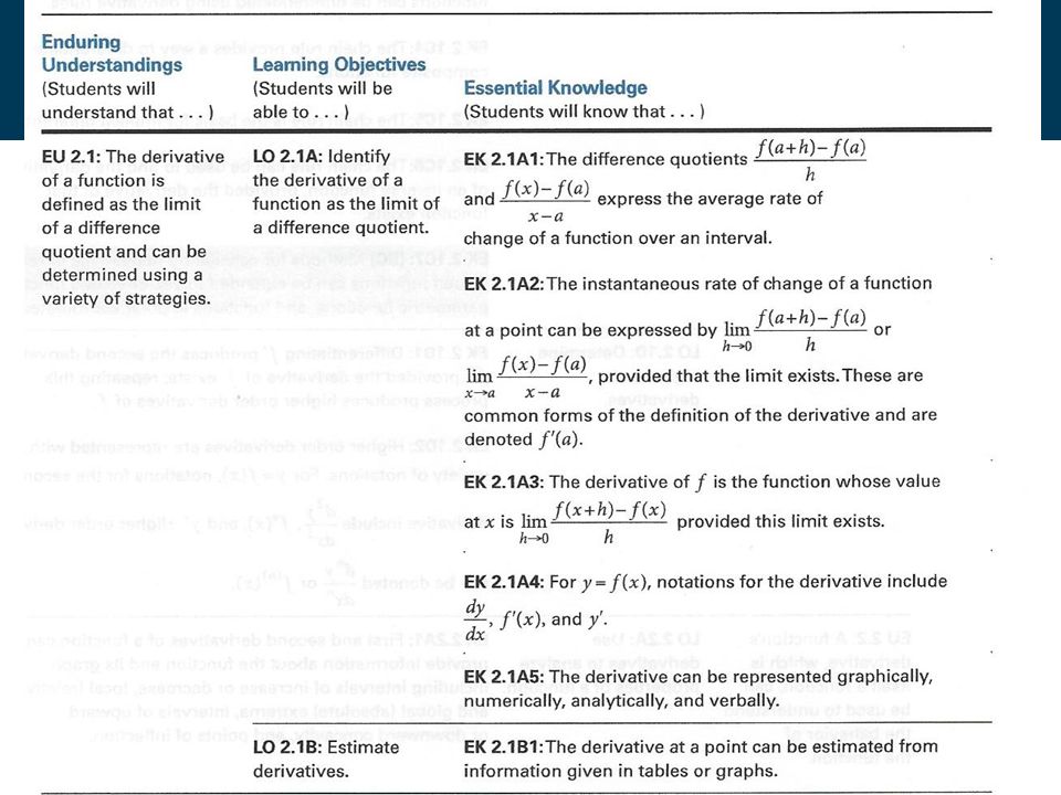
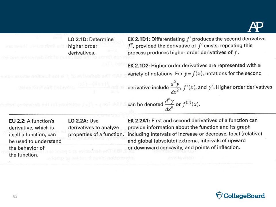
79. Big Idea 2: Derivatives
Page
Using derivatives to describe the rate of change of one variable with respect to another variable allows students to understand change in a variety of contexts.
In AP Calculus, students build the derivative using the concept of limits and use the derivative primarily to compute the instantaneous rate of change of a function.
Applications of the derivative include finding the slope of a tangent line to a graph at a point, analyzing the graph of a function (for example, determining whether a function is increasing or decreasing and finding concavity and extreme values), and solving problems involving rectilinear motion.

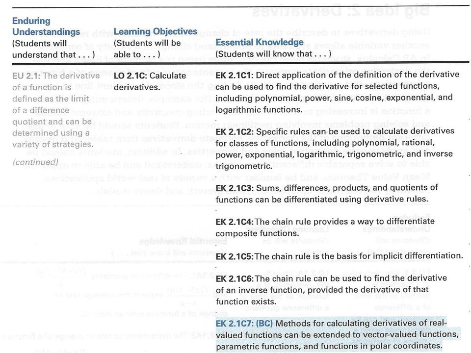
80. Big Idea 2: Derivatives
Students should be able to use different definitions of the derivative, estimate derivatives from tables and graphs, and apply various derivative rules and properties.
In addition, students should be able to solve separable differential equations, understand and be able to apply the Mean Value Theorem, and be familiar with a variety of real-world applications, including related rates, optimization, and growth and decay models.

87. Tuesday Assignment - AB
Multiple Choice Questions on the 2014 test: 9, 11, 15, 19, 21, 22, 23, 27, 28, 82, 88, 89, 90, 91, 92
Free Response:
2014: AB3, AB6
2015: AB2, AB3/BC3