1. MOBILE RADIO ENVIRONMENT AND SIGNAL DISTURBANCE

2. Introduction ..
Question:
What are reasons why wireless signals are hard to send and receive?

3. Introduction to Radio Wave Propagation
The mobile radio channel places fundamental limitations on the performance of wireless communication systems
Paths can vary from simple line-of-sight to ones that are severely obstructed by buildings, mountains, and foliage
Radio channels are extremely random and difficult to analyze
The speed of motion also impacts how rapidly the signal level fades as a mobile terminals moves about.

4. Problems Unique to Wireless systems
Interference from other service providers
Interference from other users (same network)
CCI due to frequency reuse
ACI due to Tx/Rx design limitations & large number of users sharing finite BW
Shadowing
Obstructions to line-of-sight paths cause areas of weak received signal strength

5. Problems Unique to Wireless systems
Fading
When no clear line-of-sight path exists, signals are received that are reflections off obstructions and diffractions around obstructions
Multipath signals can be received that interfere with each other
Fixed Wireless Channel → random & unpredictable
must be characterized in a statistical fashion
field measurements often needed to characterize radio channel performance

6. Mechanisms that affect the radio propagation ..
Reflection
Diffraction
Scattering
In urban areas, there is no direct line-of-sight path between:
the transmitter and the receiver, and where the presence of high- rise buildings causes severe diffraction loss.
Multiple reflections cause multi-path fading

7. Reflection, Diffraction, Scattering
Reflections arise when the plane waves are incident upon a surface with dimensions that are very large compared to the wavelength
Diffraction occurs according to Huygens's principle when there is an obstruction between the transmitter and receiver antennas, and secondary waves are generated behind the obstructing body
Scattering occurs when the plane waves are incident upon an object whose dimensions are on the order of a wavelength or less, and causes the energy to be redirected in many directions.

8. Mobile Radio Propagation Environment
The relative importance of these three propagation mechanisms depends on the particular propagation scenario.
As a result of the above three mechanisms, macro cellular radio propagation can be roughly characterized by three nearly independent phenomenon;
Path loss variation with distance (Large Scale Propagation )
Slow log-normal shadowing (Medium Scale Propagation )
Fast multipath fading. (Small Scale Propagation )
Each of these phenomenon is caused by a different underlying physical principle and each must be accounted for when designing and evaluating the performance of a cellular system.

9. Path Loss: Models of "large-scale effects"
location 1, free space loss (Line of Sight) is likely to give an accurate estimate of path loss.
location 2, a strong line-of-sight is present, but ground reflections can significantly influence path loss. The plane earth loss (2-Ray Model) model appears appropriate.

10. location 3, plane earth loss needs to be corrected for significant diffraction losses, caused by trees cutting into the direct line of sight.
location 4, a simple diffraction model is likely to give an accurate estimate of path loss.
location 5, loss prediction fairly difficult and unreliable since multiple diffraction is involved

11. Radio Propagation Mechanisms1 2 3 4
Line Of Sight (LOS)
Non Line Of Sight (NLOS)

12. Line of Sight (LOS)
Line-of-sight is the direct propagation of radio waves between antennas that are visible to each other.
The received signal is directly received at the receiver the effects such as reflection, diffraction and scattering doesn’t affect the signal reception that much.
Radio signals can travel through many non-metallic objects, radio can be picked up through walls. This is still line-of-sight propagation.
Examples would include propagation between a satellite and a ground antenna or reception of television signals from a local TV transmitter.

13. Free Space Propagation Model
Free space propagation model is used to predict:
Received Signal Strength when the transmitter and receiver have a clear, unobstructed LoS between them.
The free space propagation model assumes a transmit antenna and a receive antenna to be located in an otherwise empty environment. Neither absorbing obstacles nor reflecting surfaces are considered. In particular, the influence of the earth surface is assumed to be entirely absent.
Satellite communication systems and microwave line-of-sight radio links typically undergo free space propagation.

14. Free Space Propagation Model
Path Loss
Signal attenuation as a positive quantity measured in dB and defined as the difference (in dB) between the effective transmitter power and received power.
Friis is an application of the standard “Free Space Propagation Model “
It gives the Median Path Loss in dB ( exclusive of Antenna Gains and other losses )

15. Friis Transmission Equation (Far field)
clear, unobstructed line-of-sight path → satellite and fixed microwave

16. Friis Free Space Equation
Pt Transmitted power,
Pr(d) Received power
Gt Transmitter antenna gain,
Gr Receiver antenna gain,
d T-R separation distance (m)
L System loss factor not related to propagation system losses (antennas, transmission lines between equipment and antennas, atmosphere, etc.)
L = 1 for zero loss
Signal fades in proportion to d2

17. Friis Free Space Equation
The ideal conditions assumed for this model are almost never achieved in ordinary terrestrial communications, due to obstructions, reflections from buildings, and most importantly reflections from the ground.
The Friis free space model is only a valid predictor for “Pr ” for values of “d” which are in the far-field of the “Transmitting antenna

18. Free Space Propagation Model
Thus in practice, power can be measured at d0 and predicted at d using the relation
where d>= d0 >= df
df is Fraunhofer distance which complies:
df =2D2/
where D is the largest physical linear dimension of the antenna

19. Typically Path Loss Exponents

20. Example 1
Find the far-field distance for an antenna with maximum dimension of 1 m and operating frequency of 900 MHz.
Given;
Largest dimension of antenna, D = 1m
Operating freq, f = 900MHz,
Far-field distance

21. Example 2
(a) If a transmitter produces 50 watts of power, express the transmit power in units of dBm, and dBW.
(b) If 50 watts is applied to a unity gain antenna with a 900 MHz carrier frequency, find the received power in dBm at a free space distance of 100 m from the antenna, What is Pr (10 km)? Assume unity gain for the receiver antenna.

22. Solution
(a) TX power in dBm = 10 log10 (Pt/1mW)
= 10 log10 (50/1mW)=47 dBm
Tx power in dBW = 10 log10 (Pt/1W)
= 10 log10(50)=17 dBW
(b)
Rx power = Pr(d) = Pt Gt Gr 2 / (4)2 d2 L
Wavelength,  = , GT=Gr = 1, D=100 m, L=1
Pr(100 m) = x10-06 W = 3.5x10-3 mW =10log (3.5*10-3) = dBm
Pr(10*1000 m) = 3.5*10-3 /10^4 = 3.5*10-7 mW

23. Multipath Propagation (NLOS)
Signal arrives at Rx through different paths
Paths could arrive with different gains, phase, & delays
Small distance variation can have large amplitude variation
Physical Phenomena behind Multipath Propagation
Reflection (R), Diffraction (D), Scattering (S)

24. Small Scale Multipath fading
Multipath creates small scale fading effects:
Rapid changes in signal strength over a small travel distance or time interval
Random frequency modulation due to varying Doppler shifts on different multipath signals
Time dispersion (echoes) caused by multipath propagation delays

25. Factors influence small scale fading
Multipath propagation – result in multiple version of transmitted signal
Speed of mobile – result in random frequency modulation due to different Doppler shifts
Speed of surrounding – if the surrounding objects move at a greater rate than the mobile
The transmission bandwidth of the signal – if the transmitted radio signal bandwidth is greater than the bandwidth of the multipath channel

26. Physical Phenomena for Multipath
Reflection - occurs when signal encounters a surface that is large relative to the wavelength of the signal
Diffraction - occurs at the edge of an impenetrable body that is large compared to wavelength of radio wave. (Waves bending around sharp edges of objects)
Scattering – occurs when incoming signal hits an object whose size is in the order of the wavelength of the signal or less

27. Reflections
Reflection occurs when RF energy is incident upon a boundary between two materials (e.g. air/ground) with different electrical characteristics
Example: reflections from earth and buildings
These reflections may interfere with the original signal constructively or destructively

28. Reflections
Upon reflection or transmission, a ray attenuates by factors that depend on the frequency, the angle of incidence, and the nature of the medium (its material properties, thickness homogeneity, etc.)
The amount of reflection depends on the reflecting material.
Smooth metal surfaces of good electrical conductivity are efficient reflectors of radio waves.
The surface of the Earth itself is a fairly good reflector...

29. Ground Reflection (2-Ray) Model
a model where the receiving antenna sees a direct path signal as well as a signal reflected off the ground.
In a mobile radio channel, a single direct path between the base station and mobile is rarely the only physical path for propagation
Hence the free space propagation model in most cases is inaccurate when used alone
Hence we use the 2 Ray GRM
It considers both- direct path and ground reflected propagation path between transmitter and receiver
specular - mirror-like reflection of light

30. Ground Reflection (2-Ray) Model
This was found reasonably accurate for predicting large scale signal strength over distances of several kilometers for mobile radio systems using tall towers ( heights above 50 m )

31. Ground Reflection (2-Ray) Model
Good for systems that use tall towers (over 50 m tall)
Good for line-of-sight microcell systems in urban environments
ETOT is the electric field that results from a combination of a direct line-of-sight path and a ground reflected path

32. Ground Reflection (2-Ray) Model
The maximum T-R separation distance ( In most mobile communication systems ) is only a few tens of kilometers, and the earth may be assumed to be flat.
ETOT =The total received E-field,
ELOS=The direct line-of-sight component
Eg =The ground reflected component,

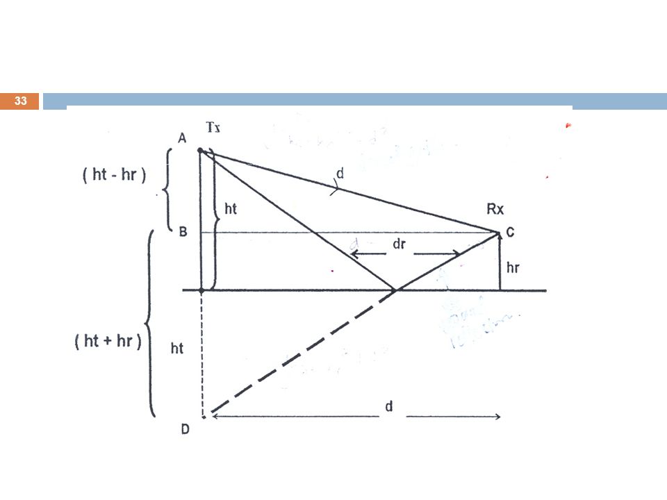
34. Triangle ABC
Binomial series, dd =
Same step for triangle BCD

35. The path difference between the reflected wave Er and direct wave Ed is
Phase difference = path different x wave number

36. Received power
Pd = power received in free space
So, power received for plane earth reflection:
Since ht, hr <<d, is small

37. Example 3
Consider GSM900 cellular radio system with 20W transmitted power from Base Station Transceiver (BTS). The gain of BTS and Mobile Station (MS) antenna are 8dB and 2dB respectively. The BTS is located 10km away from MS and the height of the antenna for BTS and MS are 200m and 3m respectively. By assuming plane earth loss between BTS and MS, calculate the received signal level at MS

38. Solution Given f = 900MHz d = 10km Pt = 20W = 43dBm ht = 200m
GT=8dB = hr = 3m
GR = 2dB = 1.58
So, the received signal at MS

39. Diffraction
Occurs when the radio path between sender and receiver is obstructed by an impenetrable body and by a surface with sharp irregularities (edges)
The received field strength decreases rapidly as a receiver moves deeper into the obstructed (shadowed) region, the diffraction field still exists and often has sufficient strength to produce a useful signal.
Diffraction explains how radio signals can travel urban and rural environments without a line-of-sight path

40. Diffraction
The phenomenon of diffraction can be explained by Huygen's principle, which states that all points on a wave front can be considered as point sources for the production of secondary wavelets, and that these 'wavelets combine to produce a new wave front in the direction of propagation
The field strength of a diffracted wave in the shadowed region is the vector sum of the electric field components of all the secondary wavelets in the space around the obstacle.

41. Scattering
The medium which the wave travels consists of objects with dimensions smaller than the wavelength and where the number of obstacles per unit volume is large – rough surfaces, small objects, foliage, street signs, lamp posts.
Generally difficult to model because the environmental conditions that cause it are complex
Modeling “position of every street sign” is not feasible.

42. Illustration ..

43. Typical large-scale path loss
Fig. 2.15
Source: Rappaport and A. Goldsmith books

44. Doppler Effect
Doppler effect occurs when transmitter and receiver have relative velocity
away
towards

45. Resting sound source Frequency fs V=340m/s Frequency fo source at rest
Wave peaks evenly spaced around the source at 1 wavelength intervals
source
at rest
observer
at rest

46. Sound source moving toward observer
Observer hears
increased pitch
(shorter wave length)
Frequency fo
Frequency fs
source
observer
at rest

47. Sound source moving away from observer
Observer hears
decreased pitch
(longer wave length)
Frequency fo
Frequency fs
observer
at rest
source

48. Doppler Shift Calculation
Δl is small enough to consider
v = speed of mobile, λ= carrier wavelength
fd is +/-ve when moving towards/away the wave
= 1

49. When they are opposing each other, the frequency decreases.
Doppler Effect: When a wave source and a receiver are moving towards each other, the frequency of the received signal will not be the same as the source.
When they are moving toward each other, the frequency of the received signal is higher than the source.
When they are opposing each other, the frequency decreases.
Doppler Shift in frequency:
where v is the moving speed,
 is the wavelength of carrier.
Moving speed v MS 
Signal

50. Example 4
Consider a transmitter which radiates a sinusoidal carrier frequency of 1850 MHz. For a vehicle moving 96 km/h, compute the received carrier frequency if the mobile is moving
(a) directly towards transmitter
(b) Directly away from the transmitter
(c) In a direction perpendicular to the direction of arrival of the transmitted signal
Solution:
fc = 1850 MHz
λ= c / f
λ = m
v = 96 km/h= m/s
(a) f = fc+ fd = MHz
(b) f = fc – fd = MHz
(c) In this case, θ =90o, cos θ = 0,
And there is no Doppler shift.
f = fc (No Doppler frequency)
Pg 180