1. Chapter 6 PHASE EQUILIBRIA
CHEM 212
Chapter 6
PHASE EQUILIBRIA
Dr. A. Al-Saadi

2. About Chapter 6 Implementing the “phase rule”.
Chapter 6 gives additional examples of and more details about equilibrium between phases.
Implementing the “phase rule”.
Applying the phase rule to:
One-component systems.
Binary systems.
Liquid-vapor equilibrium.
Temperature-composition diagrams.
Azeotropes.
Immiscible liquids.
Condensed binary systems:
Liquid-liquid systems.
Solid-liquid systems (Eutectic phase diagram).
Ternary systems.

3. The Phase Rule It was first presented by Gibbs in 1875.
It is very useful to understand the effect of intensive variables, such as temperature, pressure, or concentration, on the equilibrium between phases as well as between chemical constituents.
It is used to deduce the number of degrees of freedom (f) for a system.
The number of degrees of freedom (f) is:
The number of intensive variables that can be independently varied without changing the number of phases.
Sometimes called: “the variance of the system”.

4. The Phase Rule f = c – p + 2 The phase rule is stated as:
(f) The number of degrees of freedom is the number of intensive variables that can be independently varied without changing the number of phases.
(c) The number of components is the minimum number of independent chemical components needed to form the system or, in other words, to define all the phases.
(p) The number of phases is the number of homogeneous and distinct parts of the system separated by definite boundaries.
The number (2) is for the two intensive variables temperature and pressure.

5. Example: Phase Diagram of Water
How many components do you have?
We have only one component which is H2O.
In the one-phase regions, one can vary either the temperature, or the pressure, or both (within limits) without crossing a phase line.
We say that in these regions:
f = c – p + 2
= 1 – 1 + 2
= 2 degrees of freedom.

6. Example: Phase Diagram of Water
Along a phase line we have two phases in equilibrium with each other, so on a phase line the number of phases is 2.
If we want to stay on a phase line, we can't change the temperature and pressure independently.
We say that along a phase line:
f = c – p + 2
= 1 – 2 + 2
= 1 degree of freedom.

7. Example: Phase Diagram of Water
At the triple point there are three phases in equilibrium, but there is only one point on the diagram where we can have three phases in equilibrium with each other.
We say that at the triple point:
f = c – p + 2
= 1 – 3 + 2
= 0 degrees of freedom.

8. Phase Rule in One-Component Systems
Notice that in one-component systems, the number of degrees of freedom seems to be related to the number of phases.

9. Phase Rule in One-Component Systems
The phase rule should be applicable for any single-component systems in general.

10. Number of Components (c)
f = c – p + 2
The number of components (c) is the minimum number of independent chemical components needed to form the system or, in other words, to define all the phases.
"Independent" means:
If you have equilibrium balance between reactants and products, the number of components will be reduced by one.
If you have equal amounts (concentrations) of products formed, the number of components will also be reduced by one.

11. Number of Components (c)
f = c – p + 2
Examples (Chemical reactions):
If you have equilibrium balance between reactants and products, the number of components will be reduced by one.
If you have equal amounts (concentrations) of products formed, the number of components will also be reduced by one.
Example 1:
NaCl(s) dissolved in H2O.
Available chemical constituents are: Na+, Cl–, NaCl and H2O.
Is it correct to say c = 4 ?
Because Na+ and Cl– have the same amount “equal neutrality” as NaCl, then c = 2 and not 4.

12. Number of Components (c)
f = c – p + 2
Examples (Chemical reactions):
If you have equilibrium balance between reactants and products, the number of components will be reduced by one.
If you have equal amounts (concentrations) of products formed, the number of components will also be reduced by one.
Example 2:
CaCO3(s) CaO(s) + CO2(g)
Available chemical constituents are three.
Is it correct to say c = 3 ?
Because of the equilibrium condition the number of independent components is reduced by one. Thus, c = 2 instead of 3.

13. Number of Components (c)
f = c – p + 2
Examples (Chemical reactions):
If you have equilibrium balance between reactants and products, the number of components will be reduced by one.
If you have equal amounts (concentrations) of products formed, the number of components will also be reduced by one.
Example 2:
CaCO3(s) CaO(s) + CO2(g)
Can you specify the number of phases for the reaction?
We have here three homogeneous, distinct parts of the system separated by definite boundaries.
p = 3

14. Number of Components (c)
f = c – p + 2
Examples (Chemical reactions):
If you have equilibrium balance between reactants and products, the number of components will be reduced by one.
If you have equal amounts (concentrations) of products formed, the number of components will also be reduced by one.
Example 2:
CaCO3(s) CaO(s) + CO2(g)
So, what’s the number of degrees of freedom the system would have?
f = c – p + 2
= 2 – = 1 degree of freedom.

15. Phase Diagram of Hydrogen

16. Phase Diagram of Sulfur
Sulfur solid exists in two crystalline forms.
Orthorhombic. S8 or S(rh)
Monoclinic. S4 or S(mo)
Yellow sulfur of the orthorhombic (or rhombic) crystalline form. It is the form that commonly exists under normal conditions.

17. Phase Diagram of Sulfur

18. A More Comprehensive Phase Diagram of Sulfur

19. Liquid-Vapor Binary Systems
We need to introduce an approach that enables us to describe: the purely liquid, purely vapor, and liquid-vapor regions, as well as the boundaries between them.
Vapor
y1 , y2
Liquid
x1 , x2

20. Liquid-Vapor Binary Systems

21. Liquid-Vapor Binary Systems

22. Lever Rule, nl/nv
When the point corresponding to xtot is closer to the liquid curve, the amount of the liquid is expected to predominate as compared to that in the vapor phase.
When the point corresponding to xtot is closer to the vapor curve, the amount of the vapor is expected to predominate as compared to that in the liquid phase.
xtot
Liquid + Vapor

23. Lever Rule
xtot
Liquid + Vapor

24. Liquid-Vapor Binary Systems

25. Isothermal Distillation
This process takes place at constant temperature.
The vapor is continuously removed. As a result, the composition of the liquid phase will change. As the process is repeated more times, the concentration of the less volatile component in the liquid will increase.

26. Liquid-Vapor Equilibrium Deviating from Raoult’s Law
When Raoult’s law holds, then:
Ptot = PA + PB
The total vapor pressure value will be somewhere between the vapor pressures of the pure components.
P*B < Ptot < P*A
Liquid + Vapor

27. Liquid-Vapor Equilibrium Deviating from Raoult’s Law
When we have positive deviation from Raoult’s law, Ptot could be in some parts greater than both P*A and P*B .
As a result, a maximum in the pressure-composition curve is observed.

28. Liquid-Vapor Equilibrium Deviating from Raoult’s Law
When we have positive deviation from Raoult’s law, Ptot could be in some parts greater than both P*A and P*B .
As a result, a maximum in the pressure-composition curve is observed.

29. Liquid-Vapor Equilibrium Deviating from Raoult’s Law
When we have negative deviation from Raoult’s law, Ptot could be in some parts less than P*A and P*B .
As a result, a minimum in the pressure-composition curve is observed.

30. Liquid-Vapor Equilibrium Deviating from Raoult’s Law
When we have negative deviation from Raoult’s law, Ptot could be in some parts less than P*A and P*B .
As a result, a minimum in the pressure-composition curve is observed.

31. Binary-System Phase Diagram with Three Variables: P, T and x
The solid part of the surface represents the “liquid + vapor” region.
Above it we have the liquid phase and below it we have the vapor phase.
On the T-P planes we have pure liquid curves where the boiling point curves can be seen.

32. Binary-System Phase Diagram with Three Variables: P, T and x
On the P-x plane we have the normal pressure-composition phase diagram. It can be viewed at different temperatures.
On the T-x plane we have the temperature-composition phase diagram, which is more commonly used in experimental work since it is more convenient to fix P rather than T.

33. Temperature-Composition Phase Diagram
The T-x (isobaric) phase diagram is represented by a double curve or a lens, above which the vapor phase exists and below which the liquid phase exists, unlike the case in the P-x phase diagram.
The lowest part of the lens corresponds to the pure liquid with the highest vapor pressure “the one that vaporizes more easily”.
The opposite is true for the highest part end of the diagram.
Vapor compositions
Boiling point of liquid

34. Distillation
More commonly than using the isothermal processes, distillation process makes use of the change in the compositions in the liquid and vapor phases with the respect to temperature at constant pressure.

35. Fractional Distillation

36. Liquid-Vapor Equilibrium Deviating from Raoult’s Law
If the P-x plot shows maximum (positive deviation from Raoult’s law), the T-x plot will show a minimum.

37. Liquid-Vapor Equilibrium Deviating from Raoult’s Law
If the P-x plot shows minimum (negative deviation from Raoult’s law), the T-x plot will show a maximum.

38. Azeotropes or azeotropic mixtures
An azeotropic mixture “boiling without changing” is the mixture whose liquid and vapor phases have identical compositions of the two components.

39. Distillation of Azeotropes
You can not separate an azeotropic mixture into two pure components at the azeotropic composition.
But you can distill one pure component from the azeotropic system.
For example, boiling a mixture with a composition corresponding to p’ would produce a vapor richer with component 2 that can be condensed and re-boiled until you get pure component 2 (distillate) and a mixture (residue).

40. Distillation of Azeotropes
The same situation is applied for the minimum boiling temperature azeotrope. However, the pure component will be collected at the bottom of the fractional column (higher boiling point than the mixture).

41. Examples of Azeotropes

42. Effect of Pressure Change on Azeotropic Mixtures
With the change in pressure, not only the azeotropic boiling temperature would change (like the case for pure compounds), but also the azeotropic composition would change.

43. Immiscible Liquids
Immiscible liquids are those whose solubility within each other is so small.
At temperature T, The total pressure above such a system is simply the sum of the vapor pressures of individual components.
Vapor
Mixing
P *A
Ptot =
P *A + P *B
P *B A B
Immiscible liquids

44. Steam Distillation of Immiscible Liquids
Since:
Ptot = P *A + P *B
then the mixture is expected to boil at a temperature that is lower than the boiling point of either component.
If you want to do “steam distillation” for the system, then the relative amounts of components A and B in the vapor can be given by:
nA/nB = P *A / P *B
Because the ratio P *A / P *B is always constant at given T, then the relative amounts of A and B in the distillate at that T should be also constant.
Ptot =
P *A + P *B
Immiscible liquids

45. Immiscible Liquids

46. Partially Miscible Liquids

47. Condensed Binary Systems
In many cases, the liquid-liquid interactions are more important to be understood than the condition of liquid-vapor equilibrium.
This can be represented by having a fixed external pressure “such as a vessel open to the atmosphere”, and the solubility of the two liquids is studied as a function of temperature.

48. Condensed Binary Systems
Aniline dissolves in water (layer L1) as it is added in small amounts at any temperature below 441K.
As more aniline is added, another layer (layer L2) which is rich with aniline is formed.
The lever rule can be used to determine the compositions of the two layers. L2 L1

49. Condensed Binary Systems
As more aniline is added the amount of L2 increases on the expense of L1.
These are known as conjugate solutions.
Just right after passing point e, L1 disappears and only the aniline-rich layer exists.

50. Condensed Binary Systems

51. Condensed Binary Systems
The solubility of aniline in water and of water in aniline increases as the temperature increases for a constant composition system “Isopleths”.
The “upper consolute” temperature, Tuc, is the highest possible temperature at which the two layers can coexist or a separation can occur.

52. Condensed Binary Systems
The “upper consolute” temperature, Tuc, existence can be explained in terms of intermolecular forces. Above Tuc the forces holding the molecules close together are counteracted by the thermal motions or by the kinetic energy.

53. Condensed Binary Systems
For other systems, a lower consolute temperature (Tlc) exists.
Above Tlc, two immiscible layers exists.
Below Tlc the two liquids are miscible because they can form weak complexes (internal forces). As T increases, these weak complexes break up and immiscible systems is being formed.

54. Condensed Binary Systems
Other systems show both an upper and lower consolute temperatures.
Such systems are known as closed miscibility loops.

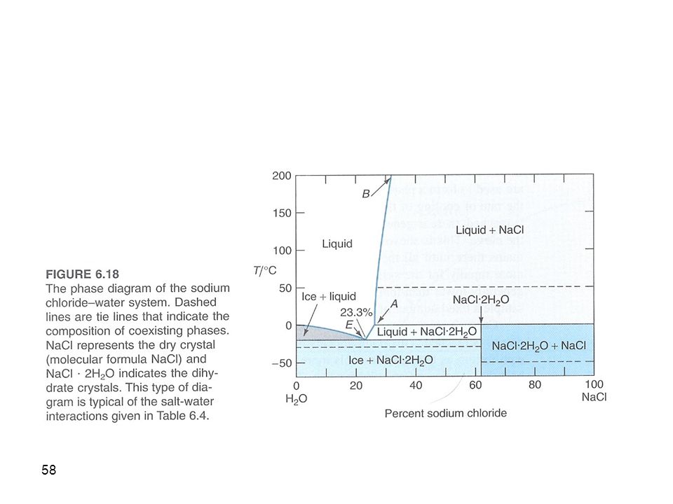
55. Zinc-Lead System
The Zn-Pb system has important metallurgical applications.