1. 7
UTILITY AND DEMAND
CHAPTER

2. Objectives After studying this chapter, you will able to
Describe preferences using the concept of utility and distinguish between total utility and marginal utility
Explain the marginal utility theory of consumer choice
Use marginal utility theory to predict the effects of changing prices and incomes
Explain the paradox of value

3. Household Consumption Choices
A household’s consumption choices are determined by:
Consumption possibilities
Preferences
Consumption Possibilities
A household’s consumption possibilities are constrained by its budget and the prices of the goods and services it buys.
A budget line describes the limits to a household’s consumption choices.

4. Household Consumption Choices
Figure 7.1 shows a budget line.
The household can afford all the points on or below the budget line.
The household cannot afford the points beyond the budget line.

6. Household Consumption Choices
Preferences
A household’s preferences determine the benefits or satisfaction a person receives consuming a good or service.
The benefit or satisfaction from consuming a good or service is called utility.
Total Utility
Total utility is the total benefit a person gets from the consumption of goods. Generally, more consumption gives more utility.

7. Household Consumption Choices
Table 7.1 on page 151 provides an example of total utility schedule.
Figure 7.2(a) shows a total utility curve.
Total utility increases with the consumption of a good.
Where do the utility numbers come from? Year after year, you will get the same question from the curious student: “where do the utility numbers come from?” This new edition tries to help with one answer to this question by telling the story of Lisa’s likes for movies and soda. We tell Lisa that we’re going to call the utility she gets from 1 movie a month 50 units of utility. Then we ask her to tell us, using the same scale, how much she would like 2, 3, and so on movies, and 1, 2, 3, and so on six-packs of soda.
A second answer that you can’t give now but you can promise when you get to the end of the chapter is that we can infer the MU values from the prices (up to an arbitrary constant of multiplication). Because in consumer equilibrium, MUM/PM = MUS/PS = , we know that MUM = PM and MUS = PS. (Use this second explanation carefully, and don’t use the math as densely as we’re using it here. Spell it out at greater length in words and with intuition.)

9. Household Consumption Choices
Marginal Utility
Marginal utility is the change in total utility that results from a one-unit increase in the quantity of a good consumed.
As the quantity consumed of a good increases, the marginal utility from consuming it decreases.
We call this decrease in marginal utility as the quantity of the good consumed increases the principle of diminishing marginal utility.

10. Household Consumption Choices
Figure 7.2(b) illustrates diminishing marginal utility.
Utility is analogous to temperature.
Both are abstract concepts and both are measured in arbitrary units.

12. Maximizing Utility
The key assumption of marginal utility theory is that the household chooses the consumption possibility that maximizes total utility.
The Utility-Maximizing Choice
We can find the utility-maximizing choice by looking at the total utility that arises from each affordable combination.
Table 7.2 (page 155) shows an example of the utility-maximizing combination, which is called a consumer equilibrium.

13. Maximizing Utility Equalizing Marginal Utility per Dollar Spent
Using marginal analysis, a consumer’s total utility is maximized by following the rule:
Spend all available income and equalize the marginal utility per dollar spent on all goods.
The marginal utility per dollar spent is the marginal utility from a good divided by its price.
MU/P
Marginal decision making is the core of the economic way of thinking. Get your students to appreciate that, aside from the concept of opportunity cost, marginal reasoning is the most important tool for understanding the economic perspective. Remind them that we have been using marginal reasoning for many chapters now:
In Chapter 2 we derived the marginal cost of production from the PPF.
In Chapter 5 we discovered that competitive equilibrium is efficient because marginal benefit on the demand curve equals marginal cost on the supply curve.
In this chapter, we discover that equating the marginal utility per dollar spent across all goods and services maximizes a consumer’s utility.

14. Maximizing Utility Call the marginal utility of movies MUM
Call the marginal utility of soda MUS
Call the price of movies PM
Call the price of soda PS
The marginal utility per dollar spent on movies is MUM/PM
The marginal utility per dollar spent on soda is MUS/PS.
People don’t calculate and compare marginal utilities and prices. One of the challenges in teaching the marginal utility theory is getting the students to appreciate the fundamental role of a model of choice. The goal is to predict choices, not to describe the thought processes that make them. The physics model of the pool player’s choices (This Instructor’s Manual, Chapter 1, p. 6) is relevant here. Gary Becker told the story a bit differently and more pointedly for present purposes. Here’s what he said (Parkin, Economics, first edition, 1990, p. 154):
Orel Hershiser [substitute a current pitcher] is a top baseball player. He effectively knows all the laws of motion, of eye and hand coordination, about the speed of the bat and ball, and so on. He’s in fact solving a complicated physics problem when he steps up to pitch, but obviously he doesn’t have to know physics to do that. Likewise, when people solve economic problems rationally they’re really not thinking that well, I have this budget and I read this textbook and I look at my marginal utility. They don’t do that, but it doesn’t mean they’re not being rational any more than Orel Hershiser is Albert Einstein.

15. Maximizing Utility Total utility is maximized when: MUM/PM = MUS/PS
Table 7.3 (page 156) and Figure 7.3 on the next slide show why the utility maximizing rule works.

16. Maximizing Utility
If MUM/PM > MUS/PS, then moving a dollar from soda to movies increases the total utility from movies by more than it decreases the total utility from soda, so total utility increases.
Only when MUM/PM = MUS/PS, is it not possible to reallocate the budget and increase total utility.

18. Maximizing Utility
Similarly, if MUS/PS > MUM/PM, then moving a dollar from movies to soda increases the total utility from soda by more than it decreases the total utility from movies, so total utility increases.
First work out what the consumer can afford. Some reviewers of this textbook have told us that we don’t need the budget line in a utility chapter and that it is only needed in an indifference curve chapter. We strongly disagree. The essence of the economic problem faced by the consumer is the economic problem of Chapter 2. The budget line is the constraint—analogous to the PPF. (Stress though that the PPF is based on technology while the budget line is based on market prices.) If you assign numerical problems on utility maximization, stress that the first step is to write down the feasible combinations. There is no point looking at combinations that the consumer can’t afford, and no point in looking at combinations that leave unspent income.
To compare marginal utility across goods requires knowledge of relative prices. Students have the most difficulty understanding why the utility maximizing rule equates the marginal utility per dollar spent rather than just plain marginal utility.
How does the consumer know how much additional utility from one good is made available when giving up some utility of the other good? Students usually grasp that the consumer must assess the marginal utility lost against the marginal utility gained as one good is substituted for another. Yet, students usually haven’t thought about how much of one good is available by forgoing some quantity of the other good. Point out that this is not known until the relative prices of the two goods are known, which is why the marginal utility is weighted by its price.
Again, only when MUM/PM = MUS/PS, is it not possible to reallocate the budget and increase total utility.

20. Predictions of Marginal Utility Theory
A Fall in the Price of a Movie
When the price of a good falls the quantity demanded of that good increases—the demand curve slopes downward.
For example, if the price of a movie falls, we know that MUM/PM rises, so before the consumer changes the quantities consumed, MUM/PM > MUS/PS.
To restore consumer equilibrium (maximum total utility) the consumer increases the quantity of movies consumed to drive down the MUM and restore MUM/PM = MUS/PS.
The concept of utility is abstract and not comparable across people—and that can be a difficult idea to grasp. Students will initially be skeptical of measuring satisfaction with the concept of utility—not because the idea that consumer satisfaction increases with consumption is difficult to comprehend, but because there is no absolute standard by which different people’s satisfaction can be compared. Many students think that if one person’s utility can’t be converted into standardized units that are comparable across people, like converting spatial distance into miles or kilometers, then the concept simply isn’t worth understanding. (In mathematical terms, utility ordering is ordinal, not cardinal, making it impossible to directly compare separate utility functions.)

21. Predictions of Marginal Utility Theory
A change in the price of one good changes the demand for another good.
You’ve seen that if the price of a movie falls, MUM/PM rises, so before the consumer changes the quantities consumed, MUM/PM > MUS/PS.
To restore consumer equilibrium (maximum total utility) the consumer decreases the quantity of soda consumed to drive up the MUS and restore MUM/PM = MUS/PS.

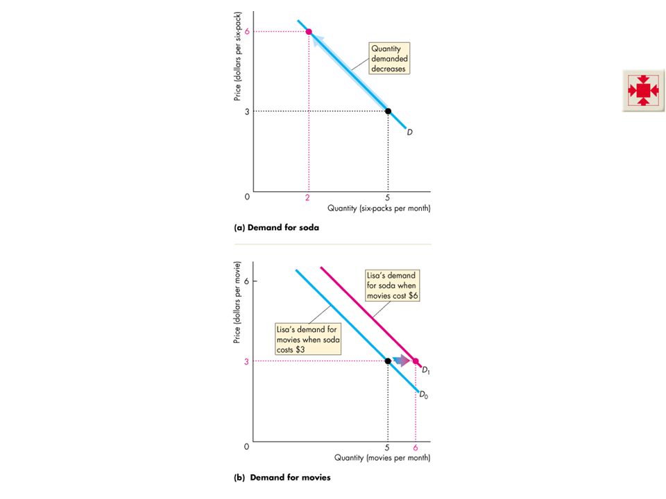
22. Predictions … Table 7.4 and Figure 7.4 illustrate these predictions.
A fall in the price of a movie increases the quantity of movies demanded—a movement along the demand curve for movies,
and decreases the demand for soda—a shift of the demand curve for soda.

24. Predictions of Marginal Utility Theory
A Rise in the Price of Soda
Now suppose the price of soda rises.
We know that MUS/PS falls, so before the consumer changes the quantities consumed, MUS/PS < MUM/PM.
To restore consumer equilibrium (maximum total utility) the consumer decreases the quantity of soda consumed to drive up the MUS and increases the quantity of movies consumed to drive down MUM. These changes restore MUM/PM = MUS/PS.

25. Predictions … Table 7.5 and Figure 7.5 illustrate these predictions.
A rise in the price of soda decreases the quantity of soda demanded—a movement along the demand curve for soda,
and increases the demand for movies—a shift of the demand curve for movies.

27. Predictions of Marginal Utility Theory
A Rise in Income
When income increases, the demand for a normal good increases.
Table 7.6 illustrate this prediction
Table 7.7 summarizes the assumptions and predictions of marginal utility theory.

28. Predictions of Marginal Utility Theory
Individual Demand and Market Demand
The market demand for a good is the relationship between the price of the good and total quantity demanded of that good.
The individual demand for a good is the relationship between the price of the good and the quantity demanded by one person.
Figure 7.6 on the next slide shows how we sum the individual demand curves to obtain the market demand.

29. Predictions of Marginal Utility Theory

30. Predictions of Marginal Utility Theory
Marginal Utility and Elasticity
We can predict the price elasticity of demand for a good by knowing the characteristics of the marginal utility of the good.
If as the quantity consumed, marginal utility diminishes rapidly, then a given price change will bring a small quantity change to restore consumer equilibrium, and demand will be inelastic.
The concept of utility is abstract, but the implications of utility analysis are concrete. Help the students be less concerned about the abstract nature of measuring utility by emphasizing that it is enough to be able to carefully analyze one consumer’s consumption decisions and extrapolate generally what this behavior could imply for market behavior in general. Appeal to those concepts that students already understand from earlier chapters by linking the abstract concept of utility with concrete implications of consumer behavior.
Mention that if utility for one good increases quickly (slowly) with consumption, this implies that an increase in the price for that good will cause only a small (large) decrease in its consumption.
This implies that as the consumer substitutes away from that good to raise the marginal utility per dollar ratio and into other goods and services to lower other marginal utility per dollar ratios, the change in quantity consumed will be relatively small (large).
The student should quickly realize that a relatively small decrease in quantity demanded due to a given increase in price indicates a relatively inelastic (elastic) demand for that good. Make the link: consumers with steep (shallow) marginal utility functions for a good must have an inelastic (elastic) demand.

31. Efficiency, Price, and Value
The Paradox of Value
The paradox of value “Why is water, which is essential to life, far cheaper than diamonds, which are not essential?” is resolved by distinguishing between total utility and marginal utility.
Figure 7.7 on the next slide illustrates the resolution of the paradox.

32. Efficiency, Price, and Value
The total utility and consumer surplus from water is large but the marginal utility and price of water is small.
In contrast, the total utility and consumer surplus from diamonds is small but the marginal utility and price of a diamond is large.

34. THE END