12 Consumer Choice and Demand

Name: 12 Consumer Choice and Demand
Uploaded: 2017-10-14T20:48:46+00:00
Duration: PTM28S41
Channel: Frank Simmons
Description: 12 Consumer Choice and Demand

12 Consumer Choice and Demand
CHAPTER Notes and teaching tips: 4, 5, 29, 41, 42, 62, 79, and 83. To view a full-screen figure during a class, click the red “expand” button. To return to the previous slide, click the red “shrink” button. To advance to the next slide, click anywhere on the full screen figure.

C H A P T E R C H E C K L I S T When you have completed your study of this chapter, you will be able to 1 Calculate and graph a budget line that shows the limits to a person’s consumption possibilities. 2 Explain the marginal utility theory and use it to derive a consumer’s demand curve. 3 Use marginal utility theory to explain the paradox of value: why water is vital but cheap while diamonds are relatively useless but expensive.

12.1 CONSUMPTION POSSIBILITIES
The Budget Line A budget line describes the limits to consumption choices and depends on a consumer’s budget and the prices of goods and services. Let’s look at Tina’s budget line: Tina has $4 a day to spend on two goods: bottled water and gum. The price of water is $1 a bottle. The price of gum is 50¢ a pack. Students are introduced to another curve in this chapter, the budget line. Remind them that this line is not a demand curve nor a production possibilities frontier. Point out the differences: A demand curve is graphed in price/quantity space and shows how the quantity demanded of a product depends on its price; a budget line is graphed in good A/good B space and shows combinations that can be afforded; and although a PPF is also graphed in good A/good B space, it applies to a nation as whole and shows what can be produced. However, the budget line is similar to the PPF because both show limits.

Figure 12.1 shows Tina’s consumption possibilities. Points A through E on the graph represent the rows of the table. To help students remember how the budget line shifts when the prices of goods change, suggest they should assume they spend ALL of their income on either good. For example, suppose apples are on the x-axis, and oranges are on the y-axis. Ask students, “What happens if the price of apples increases?” Tell them to assume that they hate apples and regardless of the price of apples, they spend their entire budget on oranges. Because the price of oranges doesn’t change, ask how the change in the price of apples impacts the number of oranges they can buy. Point out the y-intercept and stress the fact that this is the consumption point at which all their budget is spent on oranges. Make it clear that this point does not change when the price of apples rises. Then turn to the x-axis and tell students that they now buy only apples and no oranges. Discuss with them that the x-intercept shows the maximum number of apples they can buy when they spend all their budget on apples. While pointing out the x-intercept, ask students what happens to the number of apples they can buy when the price of apples rises. When they answer “fewer apples,” move your finger leftward along the x-axis and make a mark. Then draw the new budget line: the y-intercept does not change while the x-intercept rotates inward, making the budget line steeper. The point of this exercise is to focus on the intercepts and not the slope. For many students, this is an easier method of determining the change in the budget line. To complete the exercise, let the price of oranges fall and go through the same mechanics. The line passing through the points is Tina’s budget line.

The budget line separates combinations that are affordable from combinations that are unaffordable.

A Change in the Budget When a consumer’s budget increases, consumption possibilities expand. When a consumer’s budget decreases, consumption possibilities shrink.

Figure 12.2 shows the effects of changes in a consumer’s budget. An decrease in the budget shifts the budget line leftward. The slope of the budget line doesn’t change because prices have not changed.

An increase in the budget shifts the budget line rightward. Again, the slope of the budget line doesn’t change because prices have not changed.

Changes in Prices If the price of one good rises when the prices of other goods and the budget remain the same, consumption possibilities shrink. If the price of one good falls when the prices of other goods and the budget remain the same, consumption possibilities expand.

Figure 12.3 shows the effect of a fall in the price of water. On the initial budget line, the price of water is $1 a bottle (and gum is 50¢ a pack), as before.

When the price of water falls from $1 a bottle to 50¢ a bottle, the budget line rotates outward and becomes less steep.

Figure 12.4 shows the effect of a rise in the price of water. Again, on the initial budget line, the price of water is $1 a bottle (and gum is 50¢ a pack), as before.

When the price of water rises from $1 to $2 a bottle, the budget line rotates inward and becomes steeper.

Prices and the Slope of the Budget Line You’ve just seen that when the price of one good changes and the price of the other good remains the same, the slope of the budget line changes. In Figure 12.3, when the price of water falls, the budget line becomes less steep. In Figure 12.4, when the price of water rises, the budget line becomes steeper. Recall that slope equals rise over run.

Let’s calculate the slope of the initial budget line. When the price of water is $1 a bottle: Slope equals 8 packs of gum divided by 4 bottles of water. Slope equals 2 packs per bottle.

Next, calculate the slope of the budget line when water costs 50¢ a bottle. When the price of water is 50¢ a bottle: Slope equals 8 packs of gum divided by 8 bottles of water. Slope equals 1 pack per bottle.

Finally, calculate the slope of the budget line when water costs $2 a bottle. When the price of water is $2 a bottle: Slope equals 8 packs of gum divided by 2 bottles of water. Slope equals 4 packs per bottle.

You can think of the slope of the budget line as an opportunity cost. The slope tells us how many packs of gum a bottle of water costs. Another name for opportunity cost is relative price, which is the price of one good in terms of another good. A relative price equals the price of one good divided by the price of another good and equals the slope of the budget line.

12.2 MARGINAL UTILITY THEORY
Utility is the benefit or satisfaction that a person gets from the consumption of a good or service. Temperature: An Analogy The concept of utility helps us make predictions about consumption choices in much the same way that the concept of temperature helps us make predictions about physical phenomena.

Total Utility Total utility is the total benefit that a person gets from the consumption of a good or service. Total utility generally increases as the quantity consumed of a good increases. Table 12.1 shows an example of total utility from bottled water and chewing gum.

Marginal utility is the change in total utility that results from a one-unit increase in the quantity of a good consumed. To calculate marginal utility, we use the total utility numbers in Table 12.1. Once you have introduced the idea of marginal utility, ask your students why a vending machine, which requires payment for each snack purchased, is used to sell snacks while a newspaper can be sold out of a box that allows anyone to take more than one paper. If students fail to respond using marginal utility analysis, prompt them by asking, “If snacks were sold using a newspaper style box, would some people take more than they paid for?” Then ask, “Why don’t people take more than one paper?” See if the students can discover diminishing marginal utility on their own. If not, explain why different sales techniques are used: Because the marginal utility of a paper diminishes so rapidly, there is little concern that people take more than one. When you have formally taught diminishing marginal utility, tie your lecture back into this example.

The marginal utility of the third bottle of water is 36 units minus 27 units, which equals 9 units.

We call the general tendency for marginal utility to decrease as the quantity of a good consumed increases the principle of diminishing marginal utility. Think about your own marginal utility from the things that you consume. The numbers in Table 12.1 display diminishing marginal utility.

Figure 12.5 shows total utility and marginal utility. Part (a) graphs Tina’s total utility from bottled water. Each bar shows the extra total utility she gains from each additional bottle of water—her marginal utility. The blue line is Tina’s total utility curve.

Part (b) shows how Tina’s marginal utility from bottled water diminishes by placing the bars shown in part (a) side by side as a series of declining steps. The downward sloping blue line is Tina’s marginal utility curve.

Maximizing Total Utility The goal of a consumer is to allocate the available budget in a way that maximizes total utility. The consumer achieves this goal by choosing the point on the budget line at which the sum of the utilities obtained from all goods is as large as possible.

The best budget allocation occurs when a person follows the utility-maximizing rule: 1. Allocate the entire available budget. 2. Make the marginal utility per dollar equal for all goods.

Allocate the Available Budget The available budget is the amount available after choosing how much to save and how much to spend on other items. Tina has already committed most of her income to other goods and saving. Tina has an available budget of $4 a day.

Step 1: Make a table that shows the quantities of the two goods that just use all the available budget. Each row shows an affordable combination.

Equalize the Marginal Utility Per Dollar Step 2: Make the marginal utility per dollar equal for both goods. Marginal utility per dollar is the marginal utility from a good relative to the price paid for the good.

To calculate marginal utility per dollar, we divide the marginal utility from a good by its price. For example, at $1 a bottle, Tina buys 1 bottle of water and her marginal utility from bottled water is 15 units. So Tina’s marginal utility per dollar from bottled water is 15 units divided by $1, which equals 15 units per dollar. When you use the marginal utility per dollar approach to explain utility maximization, you should be prepared for students’ questioning the reality of the idea that they actually equate marginal utility per dollar before making a consumption decision. Some will say, “I’ve never calculated the marginal utility of any item I’ve ever purchased. This material doesn’t make any sense.” You should agree with your students that people don’t calculate and compare marginal utilities and prices but point out to them that the goal is to predict choices, not to describe the thought processes that make them. Indeed, one of the challenges in teaching the marginal utility theory is getting the students to appreciate the fundamental role of a model of choice. Gary Becker had a pertinent story you can use: Orel Hershiser [substitute a current pitcher] is a top baseball player. He effectively knows all the laws of motion, of eye and hand coordination, about the speed of the bat and ball, and so on. He’s in fact solving a complicated physics problem when he steps up to pitch, but obviously he doesn’t have to know physics to do that. Likewise, when people solve economic problems rationally they’re really not thinking that well, I have this budget and I read this textbook and I look at my marginal utility. They don’t do that, but it doesn’t mean they’re not being rational any more than Orel Hershiser is Albert Einstein.

Suppose that Tina allocates her budget such that the marginal utility per dollar from gum is greater than her marginal utility per dollar from water. Is Tina maximizing her total utility? Students usually grasp the consumer must assess the marginal utility lost against the marginal utility gained as one good is substituted for another. Yet, students usually haven’t thought about how much of one good is available from forgoing some quantity of the other good. Point out that this is not known until the relative prices of the two goods are known, which is why the marginal utility is weighted by its price.

No. She is not maximizing total utility. If Tina buys more gum and less water, her marginal utility from gum will decrease and her marginal utility from water will increase.

If Tina increases the amount of gum she buys and decreases the amount of water she buys until her marginal utility from gum and water are equal, she will maximize her total utility.

Step 3: Make a table that shows the marginal utility per dollar for the two goods for each affordable combination.

Row C shows the utility-maximizing quantities of water and gum.

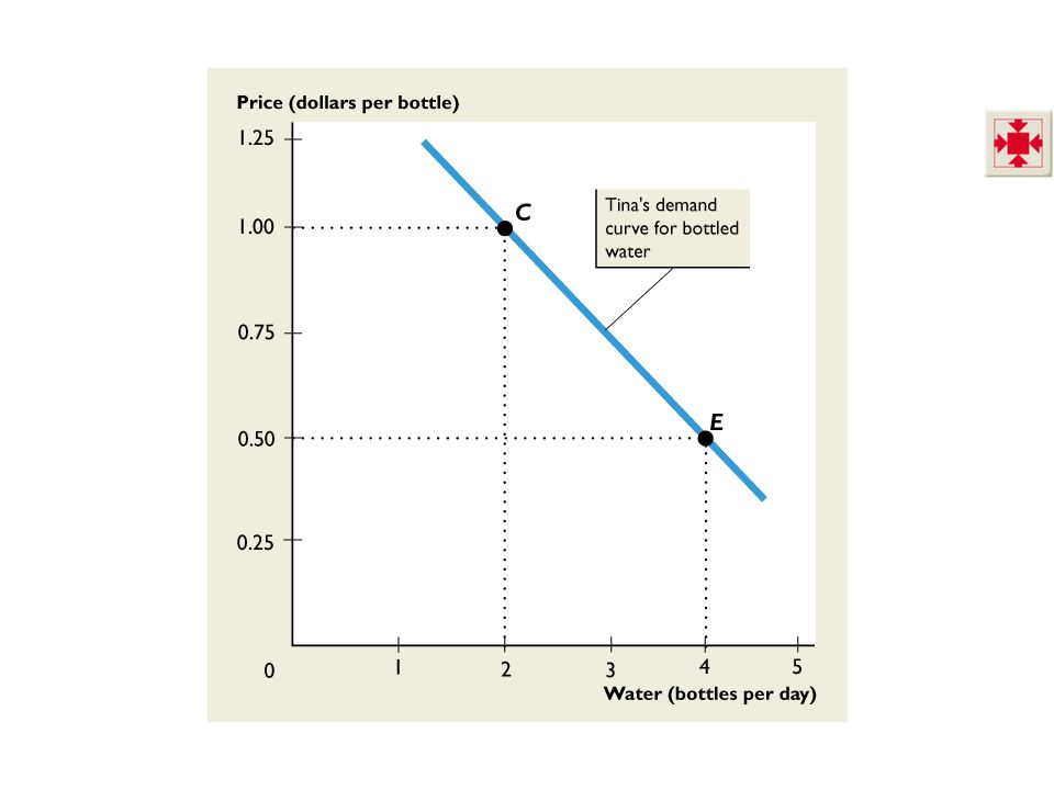
Finding an Individual Demand Curve We have found one point on Tina’s demand curve for water: When her budget is $4 a day, water is $1 a bottle and gum is 50¢ a pack, Tina buys 2 bottles of water. To find another point on her demand curve for water, let’s change the price of water to 50¢ a bottle.

A fall in the price of water increases the marginal utility per dollar from water, so Tina buys more water. Table 12.4 shows Tina’s affordable combinations of water and gum when water is 50¢ a bottle.

Row E shows Tina’s utility-maximizing quantities of water and gum. That is, when water is 50¢ a bottle (budget is $4 a day and gum is 50¢ a pack), Tina buys 4 bottles.

Figure 12.7 shows Tina’s demand curve for bottled water when her budget is $4 a day and gum is 50¢ a pack. When water is $1 a bottle, Tina buys 2 bottles and is at point C. When water falls to 50¢ a bottle, Tina buys 4 bottles and moves to point E.

The Power of Marginal Analysis The rule to follow is simple: If the marginal utility per dollar for water exceeds the marginal utility per dollar for gum, buy more water and less gum. If the marginal utility per dollar for gum exceeds the marginal utility per dollar for water, buy more gum and less water. More generally, if the marginal gain from an action exceeds the marginal loss, take the action.

Units of Utility In calculating Tina’s utility-maximizing choice in Table 12.3, we have not used the concept of total utility. All our calculations use marginal utility and price. Changing the units of utility doesn’t affect our prediction about the consumption choice that maximizes total utility.

12.3 EFFICIENCY, PRICE, AND VALUE
Consumer Efficiency When a consumer maximizes utility, the consumer is using her or his resources efficiently. Using what you’ve learned, you can now give the concept of marginal benefit a deeper meaning. Marginal benefit is the maximum price a consumer is willing to pay for an extra unit of a good or service when total utility is maximized.

The Paradox of Value For centuries, philosophers have been puzzled by the fact that water is vital for life but cheap while diamonds are used only for decoration yet are very expensive. You can solve this puzzle by distinguishing between total utility and marginal utility. Total utility tells us about relative value; marginal utility tells us about relative price.

When the high marginal utility of diamonds is divided by the high price of a diamond, the result is a number that equals the low marginal utility of water divided by the low price of water. The marginal utility per dollar spent is the same for diamonds as for water. Consumer Surplus Consumer surplus measures value in excess of the amount paid.

Figure 12.8 shows the paradox of value. The demand curve D shows the demand for water. The demand curve and the supply curve S determine the price of water at PW and the quantity at QW. The consumer surplus from water is the area of the large green triangle.

In this figure, the demand curve D is the demand for diamonds. The demand curve and the supply curve S determine the price of a diamond at PD and the quantity at QD. The consumer surplus from diamonds is the area of the small green triangle.

APPENDIX: INDIFFERENCE CURVES
An Indifference Curve An indifference curve is a line that shows combinations of goods among which a consumer is indifferent. Students need to be told why they are studying indifference curves. Indeed, many students think indifference curves impractical and so are less than eager to study them. Motivation is necessary! One way to motivate students is by pointing out that the material will be on their test. But that is perhaps not the best way. Launch your lecture on indifference curves by reminding students that economists are social scientists. As social scientists, we are interested in humans and their behavior. Tell your students that the indifference curve theory you will present is one way economists have of studying people’s behavior. Point out to them that indifference curves might not seem as “practical” as, say, elasticity, but not everything a scientist does has immediate practicality.

Figure A12.1 shows Tina’s indifference curve and Tina’s preference map.

In part (a), Tina is equally happy consuming at any point along the green indifference curve.

Point C is neither better nor worse than any other point along the indifference curve.

Points below the indifference curve are worse than points on the indifference curve—are not preferred.

Points above the indifference curve are better than points on the indifference curve—are preferred.

Part (b) shows three indifference curves—I0, I1, and I2—that are part of Tina’s preference map.

The indifference curve in part (a) is curve I1 in part (b). Tina is indifferent between points C and G.

Tina prefers point J to point C or point G. And she prefers either point C or point G to any point on curve I0.

Marginal Rate of Substitution The marginal rate of substitution is the rate at which a person will give up good y (the good measured on the y-axis) to get more of good x (the good measured on the x-axis) and at the same time remain on the same indifference curve. Diminishing marginal rate of substitution is the general tendency for the marginal rate of substitution to decrease as the consumer moves down along the indifference curve, increasing consumption of good x and decreasing consumption of good y.

Figure A12.2 shows the calculation of the marginal rate of substitution. The marginal rate of substitution (MRS) is the magnitude of the slope of an indifference curve. First, we’ll calculate the MRS at point C.

Draw a straight line with the same slope as the indifference curve at point C. The slope of this red line is 8 packs of gum divided by 4 bottles of water, which equals 2 packs of gum per bottle of water.

This number is Tina’s marginal rate of substitution. Her MRS = 2. At point C, when she consumes 2 bottles of water and 4 packs of gum, Tina is willing to give up gum for water at the rate of 2 packs of gum per bottle of water.

Now calculate Tina’s MRS at point G. The red line at point G tells us that Tina is willing to give up 4 packs of gum to get 8 bottles of water. Her marginal rate of substitution at point G is 4 divided by 8, which equals 1 ⁄2.

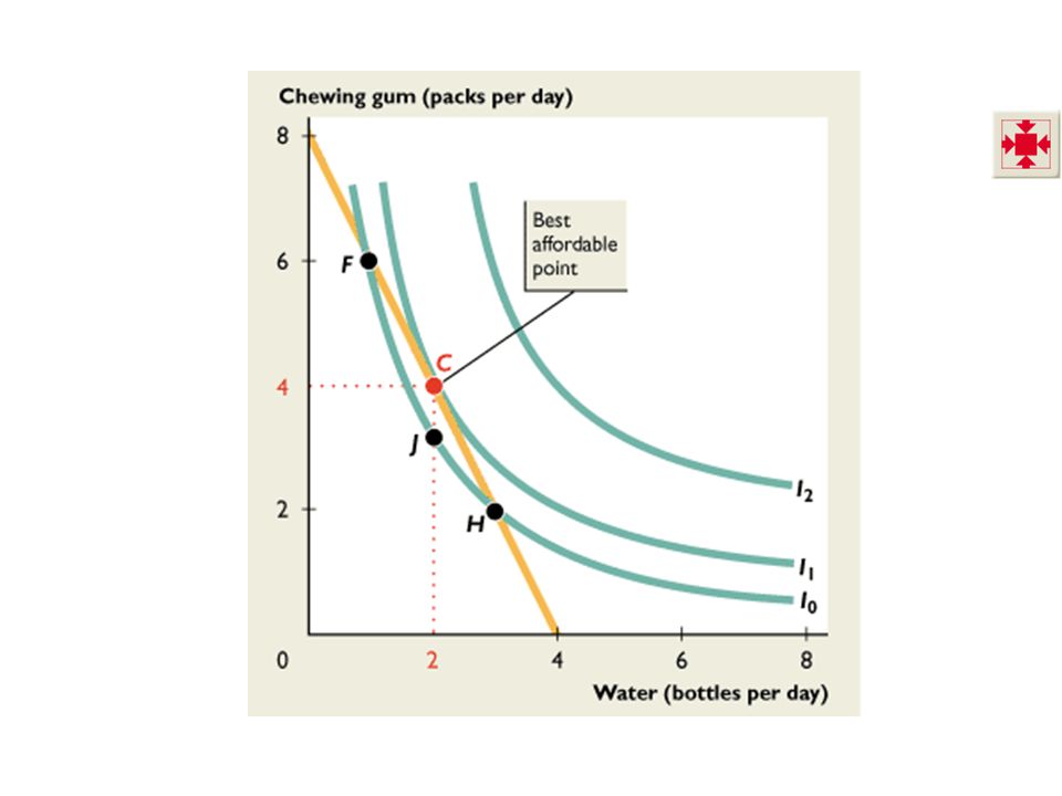
Consumer Equilibrium The goal of the consumer is to buy the affordable quantities of goods that make the consumer as well off as possible. The consumer’s preference map describe the way a consumer values different combinations of goods. The consumer’s budget and the prices of the goods limit the consumer’s choices.

Figure A12.3 shows consumer equilibrium. Tina’s indifference curves describe her preferences. Tina’s budget line describes the limits on her choice. Emphasize to the students the meaning behind the tangency point between the indifference curve and the budget line: The marginal rate of substitution (MRS) shows the consumer’s willingness to give up one good to get more of the other good. The relative price of the two goods shows what the consumer must give up of one good to get more of the other good. When a consumer equates the marginal rate of substitution (MRS) with the relative price ratio, he or she leaves no unrealized gains from substituting one good for another. The consumer is just willing to give up what he or she must give up, and there are no unrealized gains from substituting one good for another. Tina’s best affordable point is C. At point C, she is on her budget line and also on the highest attainable indifference curve.

Tina can consume the same quantity of water at point J but less gum. She prefers C to J. Point J is equally preferred to points F and H, which Tina can also afford. Points on the budget line between F and H are preferred to F and H. And of all those points, C is the best affordable point for Tina.

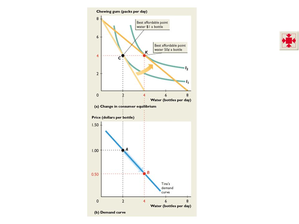
Deriving the Demand Curve To derive Tina’s demand curve for bottled water: Change the price of water Shift the budget line Work out the new best affordable point

Figure A12.4 shows how to derive Tina’s demand curve. When the price of water is $1 a bottle, Tina’s best affordable point is C in part (a) and at point A on her demand curve in part (b). A common error that students can make is to confuse the indifference curve and the demand curve. Use this derivation of the demand curve to emphasize the distinction between the two concepts. When the price of water is 50¢ a bottle, Tina’s best affordable point is K in part (a) and at point B on her demand curve in part (b).

Tina’s demand curve in part (b) passes through points A and B.

12 Consumer Choice and Demand

Similar presentations

Presentation on theme: "12 Consumer Choice and Demand"— Presentation transcript:

Similar presentations

About project

Feedback

Log in

Auth with social network:

12 Consumer Choice and Demand

Similar presentations

Presentation on theme: "12 Consumer Choice and Demand"— Presentation transcript:

Similar presentations

About project

Feedback