1. Application of the Enthalpy Method: From Crystal Growth to Sedimentary Basins Grain Growth in Metal Solidification From W.J. Boettinger  m  10km “growth” of sediment delta into ocean Ganges-Brahmaputra Delta Vaughan Voller University of Minnesota volle001@umn.edu

2. The problem—simulate the growth of a crystal into an undercooled melt contained in an insulated cavity How does solidification proceed? Why do we get a dendritic shape? Solid-liquid interface with time The Classic Stefan Problem -with curvature dependent Phase change temperature

3. seed T 0 < 0 H = cT + fL Initial liquid at a temperature below equilibrium solidification temperature T = 0 seeded with solid at solidification temperature H = 0 + fL, 0 < f < 1 Liquid layer adjacent to seed uses latent heat to heat up to T = 0 T = T 0 < 0 Negative gradient into liquid removes residual latent heat and drives solidification If a solute is present the equilibrium temp and gradient slope will be lower—resulting in a slower advance for the solidification How does solidification proceed?

4. Why do we get a dendritic shape? Initial seed with radius  anisotropic surface energy liquidus slope T o < T m Surface of seed is under-cooled due to curvature (Gibbs-Thompson) and solute (Not Shown kinetic) Capillary length ~10 -9 for metal With dimensionless numbers Angle between normal and x-axis 0.25 1 Anisotropic term makes under cooling less in preferred growth directions As crystal grows the sharper temp grad at tip drives sol harder BUT the increased tip curvature holds it back A steady tip operating Velocity is reached

5. Alain Karma and Wouter-Jan Rappel Phase Filed Current Approaches (Pure Melt) Thermodynamic equation –minimizing free energy across a diffusive interface -1 < phase marker < 1 Heat equation with source H. S. Udaykumar, R. Mittal, Wei Shyy Interface Tracking Juric Tryggvason Zhao and Heinrich Kim, Goldenfeld, Dantzig And Chen, Merriman, Osher,andSmereka Level Set Solve for level set Using speed function from Stefan Cond. Maintain distance function properties by re-in Solve heat con. Use level set to mod FD at interface

6. Enthalpy Method-First Proposed by Eyres et al 1947 For Crystal Growth by K H Tacke, 1988 A function of f if 0 < f < 1 (f determines curvature) In this work: use iterative sol. Include anisotropy and solute 0.6 0.70.3 0.0 1.0 liquid fraction 0 in solid 1 in liquid-a physical level set

7. Governing Equations With additional dimensional numbers Governing equations are Chemical potential Continuous at interface concentration If 0 < g < 1

8. In a time step Solve for H and C (explicit time integration) Calculate curvature and orientation from current nodal g field Calculate interface undercooling If 0 < g < 1 then Update f from enthalpy as Check that calculated liquid fraction is in [0,1] Update Iterate until At end of time step—in cells that have just become all solid introduce very small solid seed in ALL neighboring cells. Required to advance the solidification Numerical Solution Use square finite difference grid, set length scale to Very Simple—Calculations can be done on regular PC Initial condition— Circle r = 2.5do Typical grid Size 200x00 ¼ geometry ON A FIXED UNIFORM GRID

9. Verification 1 Looks Right!! k = 0 (pure),  = 0.05, T 0 = -0.65,  x = 3.333d 0 Enthalpy Calculation Dimensionless time  = 0 (1000) 6000 k = 0 (pure),  = 0.05, T 0 = -0.55,  x = d 0 Level Set Kim, Goldenfeld and Dantzig Dimensionless time  = 37,600

10. Verification 2 Verify solution coupling by Comparing with one-d solidification of an under-cooled binary alloy Constant T i, C i k = 0.1, Mc = 0.1, T 0 = -.5, Le = 1.0 Compare with Analytical Similarity Solution—Rubinstein Carslaw and Jaeger combo. Concentration and Temperature at dimensionless time t =100 Symbol-numeric sol. Front Movement Red-line Numeric sol. Covers analytical

11. Verification 3 Compare calculated dimensionless tip velocity with Steady state operating state calculated from the microscopic solvability theory

12. Verification 4 Check for grid anisotropy Solve with 4 fold symmetry twisted 45 o Then Twist solution back  x =.36do  x =.38do Dimensionless time  = 6000

13. k = 0.15, Mc = 0.1, T 0 = -.65  = 0.05,  x = 3.333d 0 Result: Effect of Lewis Number All predictions at Dimensionless time  =6000

14. k = 0.15, Mc = 0.1, T 0 = -.55, Le = 20.0  = 0.02,  x = 2.5d 0 Dimensionless time  = 30,000 Result: Prediction of Concentration

15. Conclusion –Score card for Dendritic Growth Enthalpy Method (extension of original work byTacke) Ease of CodingExcellent CPUVery Good (runs shown here took between 30 minutes and 2 hours on a regular PC) Convergence to known analytical sol. Excellent Convergence to known operating state Good (further study with finer grid required) Grid AnisotropyReasonable (further study with finer grid required) Flexibility to add more physics Excellent (adding solute only required 10% more lines)

16. Fans Toes Shoreline Two Sedimentary Moving Boundary Problems of Interest Moving Boundaries in Sediment Transport

17. NCED’s purpose: to catalyze development of an integrated, predictive science of the processes shaping the surface of the Earth, in order to transform management of ecosystems, resources, and land use The surface is the environment!

18. Research fields Geomorphology Hydrology Sedimentary geology Ecology Civil engineering Environmental economics Biogeochemistry Who we are: 19 Principal Investigators at 9 institutions across the U.S. Lead institution: University of Minnesota

19. 1km Examples of Sediment Fans Moving Boundary How does sediment- basement interface evolve Badwater Deathvalley

20. Sediment mass balance gives Sediment transported and deposited over fan surface by fluvial processes From a momentum balance and drag law it can be shown that the diffusion coefficient is a function of a drag coefficient and the bed shear stress  when flow is channelized = cont. Convex shape

21. sediment h(x,t) x = u(t) bed-rock ocean x shoreline x = s(t) land surface   A Sedimentary Ocean Basin

22. An Ocean Basin Melting vs. Shoreline movement

23. Experimental validation of shoreline boundary model ~3m

24. Base level Measured and Numerical results ( calculated from 1 st principles) 1-D finite difference deforming grid vs. experiment +Shoreline balance

25. An Ocean Basin Melting vs. Shoreline movement

26. Limit Conditions: A Fixed Slope Ocean q=1   s(t)  similarity solution  Enthalpy Sol. A Melting Problem driven by a fixed flux with SPACE DEPENDENT Latent Heat L =  s Depth at toe

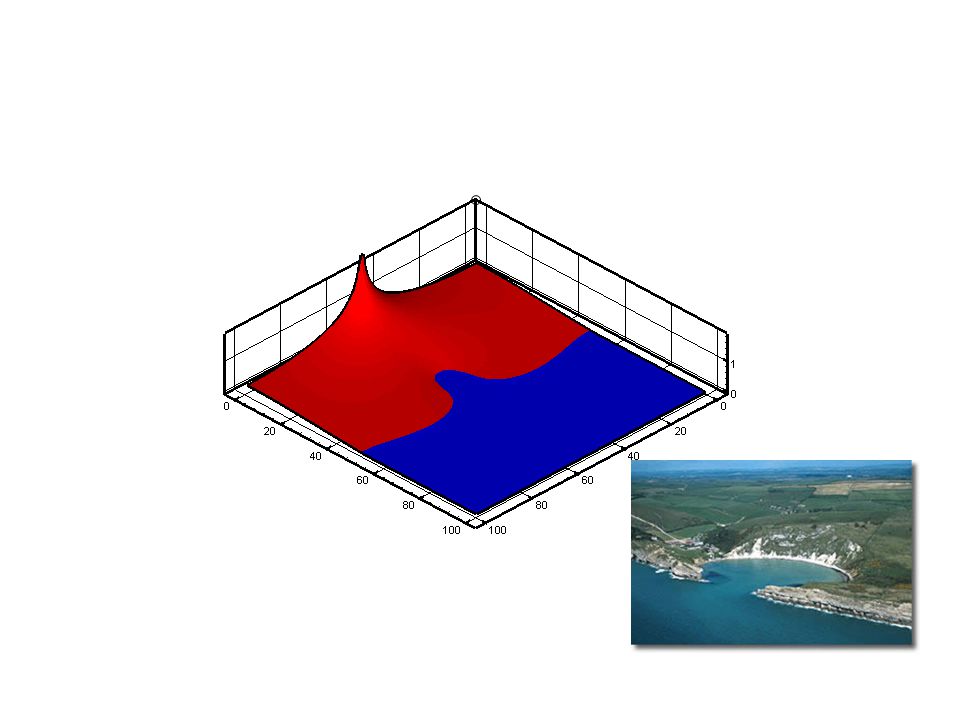
27. h(x,y,t) bed-rock ocean y shoreline x = s(t) land surface  (x,y,t) A 2-D Front -Limit of Cliff face Shorefront But Account of Subsidence and relative ocean level Enthalpy Sol. x y Solve on fixed grid in plan view Track Boundary by calculating in each cell

28.  s(t)   Hinged subsidence

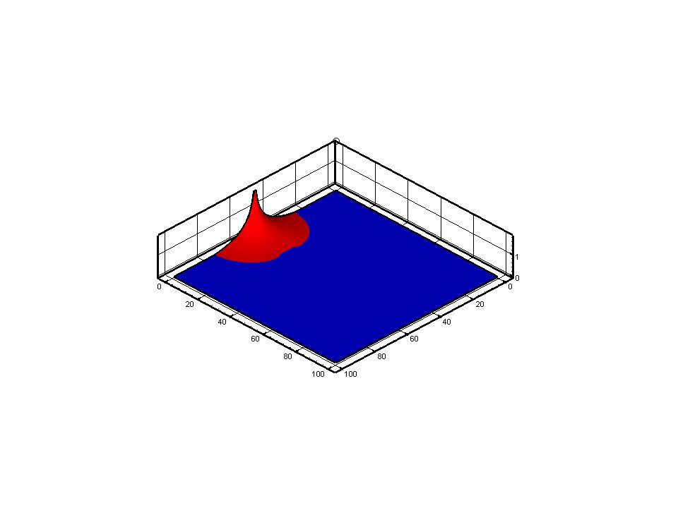
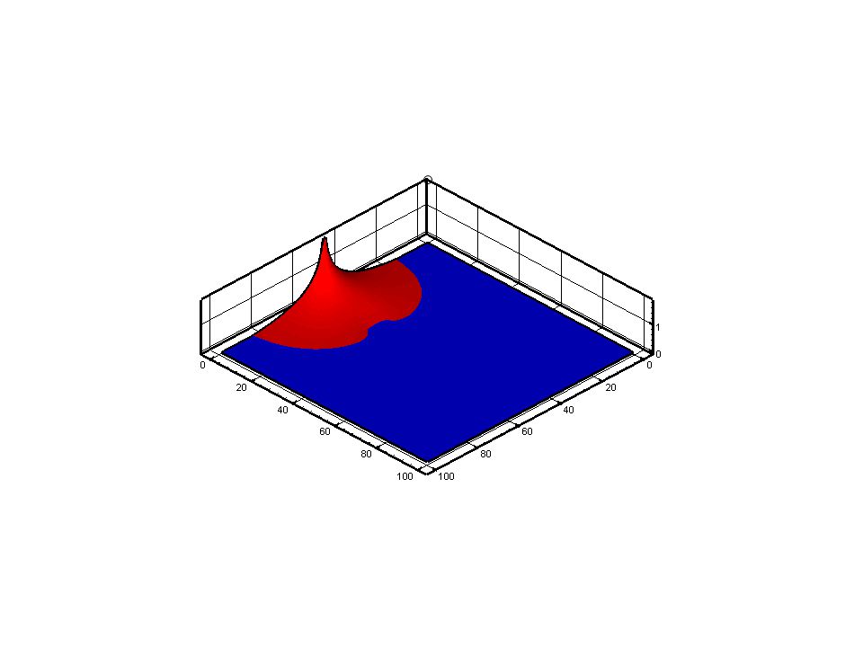
29. A 2-D problem Sediment input into an ocean with an evolving trench driven By hinged subsidence

30. With Trench

35. No Trench Trench Plan view movement of fronts

36. Models can predict stratigraphy “sand pockets” = OIL The Po Shoreline position is signature of channels WHY Build a model

37. Shoreline Tracking Model has been Latent Heat a function of Space and time Enthalpy methods can generate models for distinct moving boundary systems Crystal Growth in undercooled pure melt Phase change temperature a function of interface