1. Q 2-31 Min 3A + 4B s.t. 1A + 3B ≧ 6 B = - 1/3A + 2 1A + 1B ≧ 4

2. Objective Function Value = 3(3) + 4(1) = 13 B = - A + 4
Feasible Region
Objective Function = 3A + 4B
Optimal Solution A = 3, B = 1
Objective
Function Value
= 3(3) + 4(1) = 13
B = - 1/3A + 2 A

3. Q 2-38 a. Let S = yards of the standard grade material / frame
P = yards of the professional grade material / frame
Min 7.50S P
s.t.
0.10S P ≧ 6 carbon fiber
(at least 20% of 30 yards)
0.06S P ≦ 3 kevlar
(no more than 10% of 30 yards)
S P = 30 total
S, P ≧ 0

4. P
Total
Extreme Point
S = 10, P = 20
Feasible region is the line segment
Kevlar
Carbon fiber
Extreme Point
S = 15, P = 15 S

5. Q 2-38 c. Extreme Point Cost (15, 15) 7.50(15) + 9.00(15) = 247.50
(10, 20)
7.50(10) (20) =
>
Therefore, the optimal solution is
S = 15, P = 15

6. Q 2-38 d. Min 7.50S + 8.00P s.t. 0.10S + 0.30P ≧ 6 carbon fiber
Changing is only this value
(From 9.00 to 8.00)
Min 7.50S P
s.t.
0.10S P ≧ 6 carbon fiber
(at least 20% of 30 yards)
0.06S P ≦ 3 kevlar
(no more than 10% of 30 yards)
S P = 30 total
S, P ≧ 0
Therefore, optimal solution does not change:
S = 15, and P =15
New optimal solution value =
7.50(15) + 8(15) = $232.50

7. Q 2-38 e. At $7.40 per yard, the optimal solution is S = 10, P = 20.
So, the optimal solution is changed.
The value of the optimal solution is reduced to 7.50 (10) (20) =
A lower price for the professional grade will change the optimal solution.

8. Q 3-7 a. From figure 3.14, Optimal solution: U = 800, H = 1200
Estimated Annual Return
3(800) + 5(1200) = $8400

9. Q 3-7 b.
Constraints 1 and 2 because of 0 at Slack/Surplus column. All funds available are being fully utilized and the maximum risk is being incurred.

10. Q 3-7 c. Constraint Dual Prices Funds Avail 0.09 Risk Max 1.33
U.S. Oil Max
A unit increase in the RHS of Funds Avail makes 0.09 improvement in the value of the objective function. Risk Max also makes 1.33 improvement in the value of the objective function. A unit increase in the RHS of U.S. Oil Max makes no improvement in the objective function value.

11. Q 3-7 d. NO
A unit increase in the RHS of U.S. Oil Max makes no improvement in the objective function value.

12. Q 3-10 a. From figure 3.16, Optimal solution: S = 4,000, M = 10,000
Estimated total risk =
8(4,000) + 3(10,000) = 62,000

13. Q 3-10 b. Variable Range of Optimality S 3.75 to No Upper Limit M
No Lower Limit to 6.4

14. Q 3-10 c, d, e, f
(c) 5(4,000) + 4(10,000) = $60,000
(d) 60,000/1,200,000 = 0.05
(e) 0.057
(f) 0.057(100) = 5.7

15. Theory of Simplex Method

16. A two-variable linear programming problem
Max
s.t.
and
For any LP problem with n decision variables, each CPF (Corner Point Feasible) solution lies at the intersection of n constraint boundaries; i.e., the simultaneous solution of a system of n constraint boundary equations.

17. Max
s.t.

18. Original Form
Augmented Form
Max
s.t.
Max
s.t.
(1)
Matrix Form
(2)

19. Matrix Form (2) is
Max
s.t.
(3) or
Max
s.t.
(4)
where

21. Then, we have
Max
s.t.
(5)
(6)
where

22. Eq. (6) becomes
(7)
Putting Eq. (7) into (5), we have
(8)
So,
(9)
(10)

23. Eq. (10) can be expressed by
(11)
From Eq. (2),
(12)

24. Thus, initial and later simplex tableau are

25. The Overall Procedure 1. Initialization: 2. Iteration:
Same as for the original simplex method.
2. Iteration:
Step 1
Determine the entering basic variable:
Same as for the Simplex method.

26. Step 2
Determine the leaving basic variable:
Same as for the original simplex method, except calculate only the numbers required to do this [the coefficients of the entering basic variable in every equation but Eq. (0), and then, for each strictly positive coefficient, the right-hand side of that equation].

27. 3. Optimality test: Step 3 Determine the new BF solution:
Derive and set
3. Optimality test:
Same as for the original simplex method, except calculate only the numbers required to do this test, i.e., the coefficients of the nonbasic variables in Eq. (0).

28. Fundamental Insight Z
RHS Z 1
Row0
Row1~N

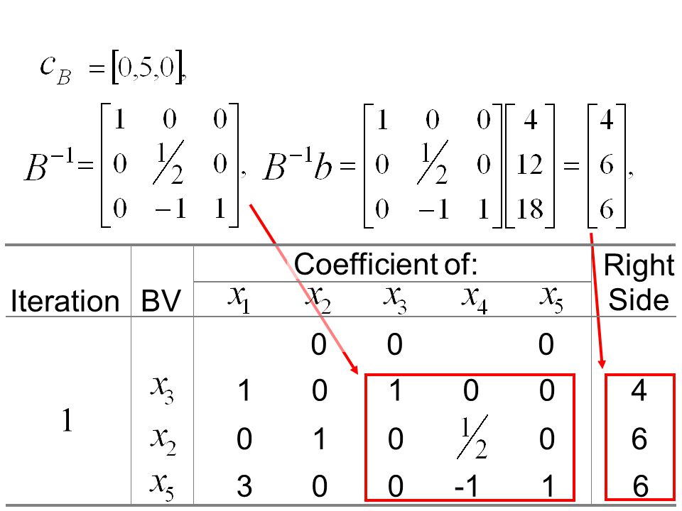
29. Coefficient of:
Right
Side
Iteration BV

30. 1 Coefficient of: Right Side Iteration BV 0 0 0 1 0 1 0 0 4 0 1 0 0 6 1

31. 1 Coefficient of: Right Side Iteration BV -3 0 0 0 1 0 1 0 0 4 1

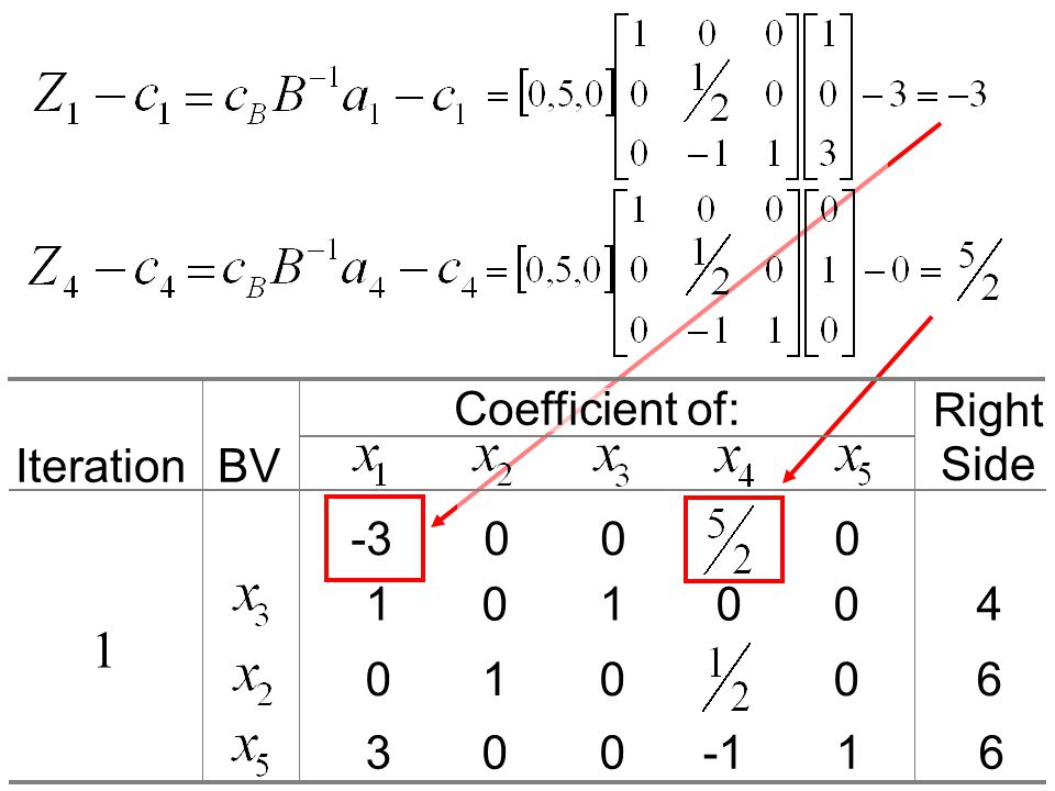
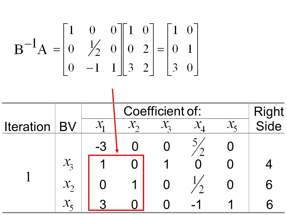
32. 1 Coefficient of: Right Side Iteration BV -3 0 0 0 1 0 1 0 0 4 1

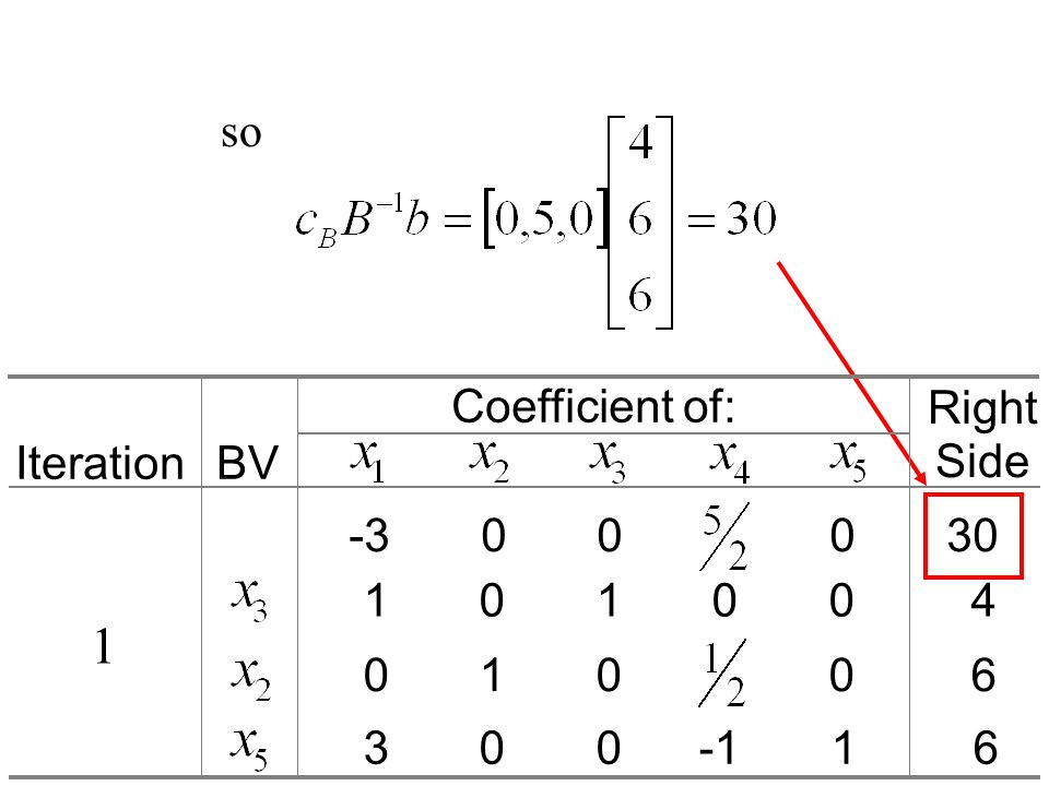
33. 1 so Coefficient of: Right Side Iteration BV -3 0 0 0 30 1 0 1 0 0 4 1

34. The most negative coefficient4 6
minimum
The most negative coefficient
Coefficient of:
Right
Side
Iteration BV 1

35. 2 Coefficient of: Right Side Iteration BV 0 0 0 0 0 1 2 0 1 0 0 6 2

36. 2 Coefficient of: Right Side Iteration BV 0 0 0 1 0 0 1 2 0 1 0 0 6 2

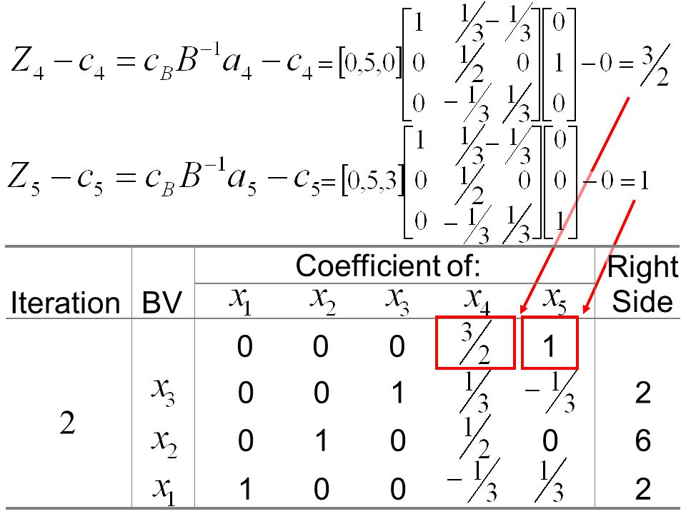
37. 2 so Coefficient of: Right Side Iteration BV 0 0 0 1 36 0 0 1 2 2

38. Duality Theory

39. One of the most important discoveries in the early development of linear programming was the concept of duality.
Every linear programming problem is associated with another linear programming problem called the dual.
The relationships between the dual problem and the original problem (called the primal) prove to be extremely useful in a variety of ways.

40. Primal and Dual Problems
Primal Problem
Dual Problem
Max
s.t.
Min
s.t.
for
for
for
for
The dual problem uses exactly the same parameters as the primal problem, but in different location.

41. In matrix notation
Primal Problem
Dual Problem
Maximize
subject to
Minimize
subject to
Where and are row vectors but and are column vectors.

42. Example
Primal Problem
Dual Problem
Max
s.t.
Min
s.t.

43. Primal Problem
in Matrix Form
Dual Problem
in Matrix Form
Max
s.t.
Min
s.t.

44. Primal-dual table for linear programming
Primal Problem
Coefficient of:
Right
Side
Coefficient
of:
Objective Function
Coefficients for
(Minimize)
Dual Problem VI VI VI
Right
Side
Coefficients for
Objective Function
(Maximize)

45. Relationships between Primal and Dual Problems
One Problem Other Problem
Constraint Variable
Objective function Right sides
Minimization
Maximization
Variables
Constraints
Unrestricted
Constraints
Variables
Unrestricted

46. The feasible solutions for a dual problem are those that satisfy the condition of optimality for its primal problem.
A maximum value of Z in a primal problem equals the minimum value of W in the dual problem.

47. Rationale: Primal to Dual Reformulation
Lagrangian Function
Max cx
s.t. Ax b
x 0
L(X,Y) = cx - y(Ax - b)
= yb + (c - yA) x
= c-yA
Min yb
s.t. yA c
y 0

48. The following relation is always maintained
yAx yb (from Primal: Ax b)
yAx cx (from Dual : yA c)
From (1) and (2), we have
cx yAx yb
At optimality
cx* = y*Ax* = y*b
is always maintained.
(1)
(2)
(3)
(4)

49. “Complementary slackness Conditions” are obtained from (4)
( c - y*A ) x* = 0
y*( b - Ax* ) = 0
xj* > y*aj = cj , y*aj > cj xj* = 0
yi* > aix* = bi , ai x* < bi yi* = 0
(5)
(6)

50. Any pair of primal and dual problems can be converted to each other.
The dual of a dual problem always is the primal problem.

51. Converted to Standard Form
Dual Problem
Min W = yb,
s.t yA c y
Max (-W) = -yb,
s.t yA -c y
Converted to
Standard Form
Its Dual Problem
Max Z = cx,
s.t Ax b x
Min (-Z) = -cx,
s.t Ax -b x

52. Min
s.t.
Min
s.t.

53. Max
s.t.
Max
s.t.

54. Home Work Ch 4: Problem 1 Ch 4: Problem 10
Additional Problems: A-1 and A-2
(See the proceeding PPS)
Due Date: September 16

55. A – 1 Theory of Simplex Method: Consider the following problem.
Let x5 and x6 denote slack variables for the two constraints. After you apply the simplex method, a portion of the final simplex tableau is as follows:

56. A – 1 cont’d Solve the problem.
Basic Variable
Coefficient of:
Right Side
Eq. Z x1 x2 x3 x4 x5 x6
(0) 1
(1) -1
(2) 2
Solve the problem.
What is B-1 ? How about B-1b and CBB-1b ?
If the right hand side is changed from (5, 4) to (5, 5), how is and optimal solution changed? How about an optimal objective value?

57. A – 2
Linear Programming: Slim-Down Manufacturing makes a line of nutritionally complete, weight-reduction beverages. One of their products is a strawberry shake which is designed to be a complete meal. The strawberry shake which is designed to be a complete meal. The strawberry shake consists of several ingredients. Some information about each of these ingredients is given below.

58. A – 2 cont’d Ingredient Calories from Fat (per tbsp)
Total Calories (per tbsp)
Vitamin Content (mg/tbsp)
Thickeners (mg/tbsp)
Cost (¢/tbsp)
Strawberry flavoring 1 50 20 3 10
Cream 75
100 8
Vitamin supplement 25
Artificial sweetener
120 2 15
Thickening agent 30 80 6

59. A – 2 cont’d
The nutritional requirements are as follows. The beverage must total between 380 and 420 calories (inclusive). No more than 20 percent of the total calories should come from fat. There must be at least 50 milligrams (mg) of vitamin content. For taste reasons, there must be at least 2 tablespoons (tbsp) of strawberry flavoring for each tablespoon of artificial sweetener. Finally, to maintain proper thickness, there must be exactly 15 mg of thickeners in the beverage.
Management would like to select the quantity of each ingredient for the beverage which would minimize cost while meeting the above requirements.

60. A – 2 cont’d Formulate a linear programming model for this problem.
Show its dual formulation.
Solve this model by your computer and confirm complementary slackness condition.