1. Linear Programming (graphical + simplex with duality) Based on Linear optimization in application by Sui lan Tang. Linear Programme (LP) for Optimization There are two methods used, namely: 1) Graphical - solving LP with 2 decision variables Starting with LP, the simpler variety of programming problems, in which the objective function as well as the constraint inequalities are all linear – with the meaning that the equations do not have exponentials. 2) Simplex: solve any number of decision variables – Primal and dual are the two terms used in LP to denote equation. For example if the primal is maximization then it is changed into minimization and vice versa. The changed equation is dual and the process is duality.

2. Simple example of linear programme (Chang, 1984) The essence of linear programming can best be conveyed by means of concrete examples: Problem of diet: To maintain good health, a person must fulfill certain minimum daily requirements of nutrients and for sake of convenience, Calcium, Protein and vitamin A. Assume that a person’s diet is to consist of only two types of food items: I and II whole price and nutrient contents are given in table 1.

4. What combination of the two food items will satisfy the daily requirement and entail the least cost? If we denote the quantities of food to be purchased each day by X 1 and X 2 (regarded as continuous variables), the problem can be stated mathematically as follows: Minimize C = 0.6 X 1 + 1 X 2

5. Subjected to10 X 1 + 4X 2 ≥ 20 (calcium constraint) 5X 1 + 5X 2 ≥ 20 (Protein constraint) 2X 1 + 6X 2 ≥ 12 (Vitamin A constraint) and X 1, X 2 ≥ 0

6. The first equation is the cost function based on price information in the table-1, constitutes the objective function of the linear program: here the function is to be minimized. The three equations that follow are the constraints necessitated by the daily requirements, these are readily translated from the last three rows of the table. Lastly, X 1, X 2 ≥ 0 referred to as non negativity constraints. Hence, there are three essential ingredients in a linear program: an objective function, a set of constraints, and a set of non negativity restrictions.

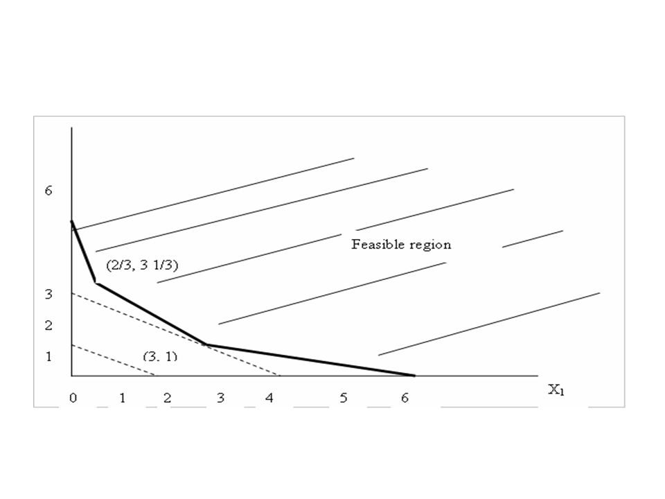
7. The graphical solution: The above mentioned problem involves only two choice variables and hence is suitable for graphical solution. Let us plot X 1 and X 2 on the two axes. Because of the non negativity restrictions, we have to consider only non negative quadrant. For the sake of convenience, we assume that three constraints are given as equations and plot them as three straight lines as given in figure -1.

10. Each of these lines (calcium, protein and vitamin A borders respectively) represent the three constraints and point (1,2) for instance satisfies the vitamin A constraint but it fails the other two. The shaded area in figure 1b is called the feasible region and each point in this region is known as a feasible solution represented by heavily kinked boundary. In particular, the set of point in the horizontal axis (x 1, x 2 ) (x 1 ≥6, x 2 = 0) as well as the set of points on the vertical axis (x 1,x 2 ) (x 1 =0, x 2 ≥5) are also members of feasible region.

11. The points (3,1) and (2/3, 3 1/3) and axix (0,5) and (6,0) are referred as extreme points which will prove of great significance in the solution. The points in the feasible region satisfy all the constraints as well as the non negativity restrictions, but some of these would entail lower purchase cost than others. We can write the cost function as: X 2 = C – 0.6 X 1 Putting C = 1 and X 2 = 0, we get -1 = -0.6 X 1 or X 1 = 1.7 Again putting X 1 = 0, then X 2 = 1 Thus we get cost line (dotted line) given in figure1b.

12. Parallel of the cost line, iso-cost line touches the extreme point at (3,1), it follows that the minimized cost of diet calculated at the food prices given will amount to : C = 3*$0.6 + 1*$1.0 = $2.8 /day

13. We can also get the same result by solving: 5x 1 + 5x 2 = 20 ------------------(i) 2x 1 + 6x 2 = 12 ------------------(ii) From (i) 5x 1 = 20-5x 2 Or x1 = (20-5x 2 )/5 ------------(iii) Putting x1 in (ii) we get 2(20-5x 2 )/5 + 6x 2 = 12 (40-10x 2 )/5 + 6X 2 = 12 Or 8 – 2x 2 + 6x 2 = 12 Or 4x 2 = 12-8 Therefore x 2 = 1 Putting value of x 2 in (iii) We get X 1 = (20-5*1)/5 = 15/5 = 3 We can find (x 1,x 2 ) = (3,1)

14. Price change: The slope of iso-cost -0.6/1.0 = -0.6 may change but there are different possibilities. First, two prices change in exactly same proportion then, the slope of iso-costs remain unchanged. In that situation, the original optimal solution continue to prevail. Second, the two prices may change in different proportion with minor difference, in such case the slope of iso-costs will undergo a small change, say from -0.6 to -0.4 or to - 0.8 by drawing a variety of a slope change of this magnitude will still leave the original optimal solution unaffected. Thus, unlike the point of tangency in differential calculus, the point of contact (the optimal corner) is insensitive to small changes in price parameters.

15. As, yet another possibility, suppose that both price now become equal, say at p 1 =p 2 =1 the lowest possible iso-cost will then contact the feasible region not at single point but along an entire edge of its boundary, with the result that each point on line segment extending from (3,1) to (2/3, 3 1/3) is equally optimal.

16. You can consider it as a blessing not a problem !!! because, it can now make possible some variation in menu. But for us, it is a retraction of our earlier statement that the optimal solutions are always to be found at extreme points – but still if we consider our attention to extreme points only, we run no risk of missing any better solution. We shall find that it is this line of thinking that underlies the so called “simplex” method of solution to be introduced later.

17. Thanks for your attention