Download presentation
Presentation is loading. Please wait.

2
Fiscal Policy and Multiplier Chapter 11 and 9 6/9/2015© 2002 Claudia Garcia-Szekely1

3
Is the government concerned with inflation? Or unemployment? To close the gap we need to increase? Or Decrease AE? and AD? Increase Taxes Decrease Transfers Decrease Government Spending Increase Taxes Decrease Transfers Decrease Government Spending Decrease AE Decrease AD

4
S Potential GDP D E B 2,000 3,000 4,000 5,000 6,000 7,000 Real GDP (billions of dollars per year) Is the government concerned with inflation? Or unemployment? To close the gap we need to increase? Or Decrease AE? and AD? Increase AE Decrease Taxes Increase Transfers Increase Government Spending Decrease Taxes Increase Transfers Increase Government Spending Increase AD

5
Fiscal Policy Changes in Government Spending, Transfers and/or Taxes. Induce a change in Aggregate Spending. Increase AE Expansionary Policy Decrease AE Contractionary Policy Decrease Taxes Increase Transfers Increase Government Spending Decrease Taxes Increase Transfers Increase Government Spending Increase Taxes Decrease Transfers Decrease Government Spending Increase Taxes Decrease Transfers Decrease Government Spending

6
Using the MPC = C/ Y 5 10002000 2250 2250+700 = 2950 a* MPC =0.7 Y = 1000 C = 700 C = Y*MPC C = 1000*0.7 ? C = Y*MPC C = Y*MPC

7
Y = AE 45 Y Firms Increase Output: hire more workers The Multiplier Y0Y0 Y 1 = Y 0 + G +sum c Y Increase Y = G + sum c c = 100*MPC Y=90 c = 90*0.9 Y=81 90 81 GG Sum C Newly employed buy more goods and services Y=100 G=100 Increase in induced consumption: Move up along C and AE AE 0 =Y 0 AE 1 =Y 1 AE Inventories Drop c = 81*0.9 Y=73 Y=66 Y=59

8
We can write the change in spending as: 100 100 * 0.9 100 * 0.9 *0.9 100 * 0.9 *0.9 *0.9 100 * 0.9 *0.9 100 * 0.9 *0.9 *0.9 *0.9 and so on…

9
100 * 0.9 Factor out 100: 100 100 * 0.9 *0.9 *0.9 100 * 0.9 *0.9 100 * 0.9 *0.9 *0.9 *0.9 100 For any increase in autonomous spending and any MPC:

10
9 To calculate the chain of spending generated from an increase in: Government Spending Investment Autonomous Consumption Net exports Autonomous Spending Multiplier:

11
45 Y The Multiplier Y0Y0 Y 1 = Y0+YY0+Y AE 0 =Y 0 AE 1 =Y 1 AE Y = G (multiplier) YY
 YY")
12
11 "We're going to be putting money in people's pockets so that they can spend on buying a new computer for their kid's school, so that they can, you know, make sure that they are able to deal with heat and groceries and all the other strains on the family budget,“ President elect, Obama. Stimulus Package = 700 Billion

13
The American Recovery and Reinvestment Act of 2009 $787.2 billion stimulus plan: the largest fiscal injection in history –$308 billion in discretionary spending –$288 billion in tax credits and incentives for individuals and –$192 billion in direct aid to states, unemployed and for the adoption of health care Information Technology 12

14
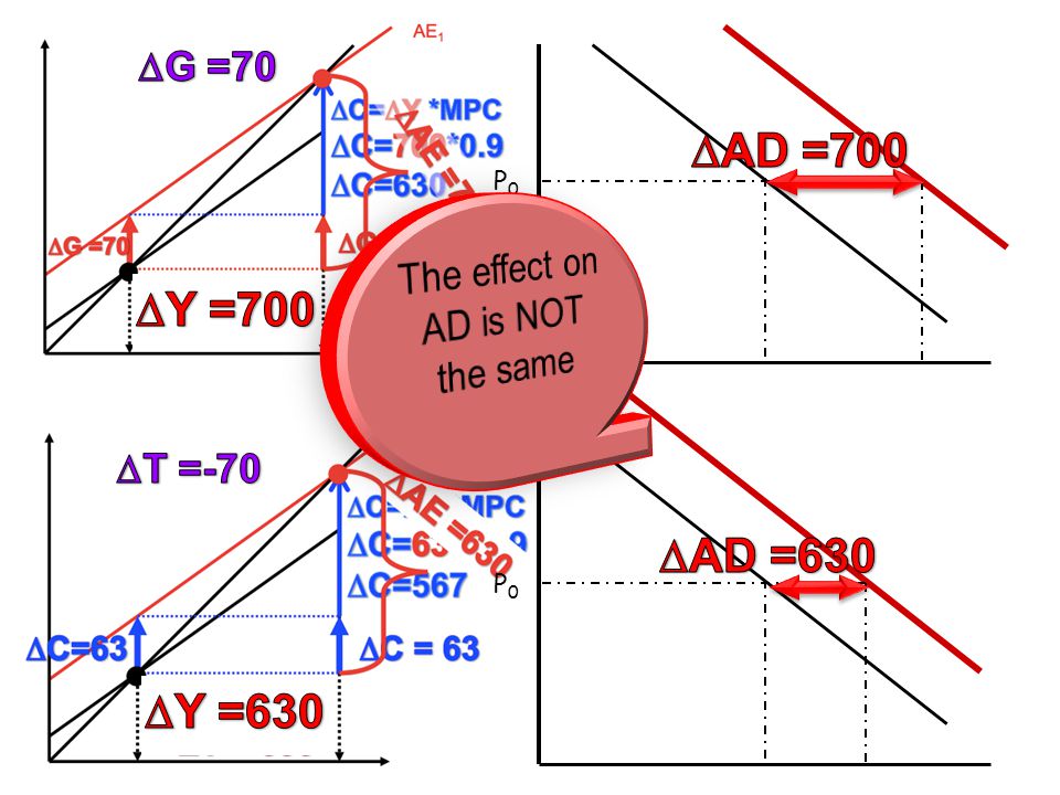
Y =Y = [ (1- 0.9) ] 1 Y = G x [ (1- MPC) ] 1 Y Y = 700 (1/0.1) = 7000 700 x A 700 increase in government spending generates a 7000 increase in output. MPC = 0.9. Effect of 700 increase in Government Spending: G = 700 AE = 700 Y = 7000 G 0 =3,000 AE 1 =C+I+G 1 +NX AE 0 =C+I+G 0 +NX G 1 =3,700 AE 1 =C+I+G 1 +NX AE 0 =C+I+G 0 +NX Change in Equilibrium Y :
![Y =Y = [ (1- 0.9) ] 1 Y = G x [ (1- MPC) ] 1 Y Y = 700 (1/0.1) = x A 700 increase in government spending generates a 7000 increase in output.](http://images.slideplayer.com/16/4894137/slides/slide_14.jpg "MPC = 0.9. Effect of 700 increase in Government Spending: G = 700 AE = 700 Y = 7000 G 0 =3,000 AE 1 =C+I+G 1 +NX AE 0 =C+I+G 0 +NX G 1 =3,700 AE 1 =C+I+G 1 +NX AE 0 =C+I+G 0 +NX Change in Equilibrium Y :.")
15
Y = 700 (1/0.1) = 7000 The shift in AD is the same as the increase in Equilibrium output: G = 700 AE = 700 Y = 7000 G 0 =3,000 AE 1 =C+I+G 1 +NX AE 0 =C+I+G 0 +NX G 1 =3,700 AE 1 =C+I+G 1 +NX AE 0 =C+I+G 0 +NX AD 1 =C+I+G 1 +NX AD 0 =C+I+G 0 +NX Y = 7000 P0P0
 = 7000 The shift in AD is the same as the increase in Equilibrium output: G = 700 AE = 700 Y = 7000 G 0 =3,000 AE 1 =C+I+G 1 +NX AE 0 =C+I+G 0 +NX G 1 =3,700 AE 1 =C+I+G 1 +NX AE 0 =C+I+G 0 +NX AD 1 =C+I+G 1 +NX AD 0 =C+I+G 0 +NX Y = 7000 P0P0")
16
6/9/2015© 2002 Claudia Garcia-Szekely15 The Multiplier Amplifies a drop in spending –As that caused by lower government spending in Iraq when the U.S. pulls troops out. Amplifies an increase in spending –As that caused by the $787 billion stimulus package.

17
6/9/2015© 2002 Claudia Garcia-Szekely16 Government Spending vs. Tax Cuts The $787 B stimulus package includes $70 billion in tax cuts, which some economists believe will not create as many new jobs as $70 billion in spending would…

18
An Increase in Government Spending AE 0 45 AE 1 Increase in Equilibrium Income:

19
6/9/2015© 2002 Claudia Garcia-Szekely18 Fixed Taxes (Lump Sum) Do not change with income: Residential Property Taxes
 Do not change with income: Residential Property Taxes")
20
6/9/2015© 2002 Claudia Garcia-Szekely19 Government Spending vs. Tax Cuts Government Spending ( G ) Enters directly into AE AE = C+I+ G Enter in directly into AE via C AE = C +I+G Taxes, transfers (T)
 Enters directly into AE AE = C+I+ G Enter in directly into AE via C AE = C +I+G Taxes, transfers (T).")
21
The effect of a tax cut

22
A decrease in Taxes AE 0 45 AE 1 Increase in Equilibrium Income:

23
AE 0 AE 1 An increase in Government Spending

25
P0P0 P0P0

26
25 Y = T [ (1- MPC) ] - (MPC) The Tax Multiplier C=- T(MPC) Y = C x [ (1- MPC) ] 1 Y = - T(MPC) x [ (1- MPC) ] 1
![25 Y = T [ (1- MPC) ] - (MPC) The Tax Multiplier C=- T(MPC) Y = C x [ (1- MPC) ] 1 Y = - T(MPC) x [ (1- MPC) ] 1](http://images.slideplayer.com/16/4894137/slides/slide_26.jpg "25 Y = T [ (1- MPC) ] - (MPC) The Tax Multiplier C=- T(MPC) Y = C x [ (1- MPC) ] 1 Y = - T(MPC) x [ (1- MPC) ] 1")
27
AE 0 AE 1

28
AE 0 AE 1

29
6/9/2015© 2002 Claudia Garcia-Szekely28 The Tax Multiplier Y = T [ (1- MPC) ] - (MPC) Y = T [- (MPS) ] (MPC)
![6/9/2015© 2002 Claudia Garcia-Szekely28 The Tax Multiplier Y = T [ (1- MPC) ] - (MPC) Y = T [- (MPS) ] (MPC)](http://images.slideplayer.com/16/4894137/slides/slide_29.jpg "6/9/2015© 2002 Claudia Garcia-Szekely28 The Tax Multiplier Y = T [ (1- MPC) ] - (MPC) Y = T [- (MPS) ] (MPC)")
30
The Tax Multiplier Formula A negative Number! A negative Number! Taxes and Output move in opposite directions Y = T [ (1- MPC) ] - (MPC)
 ] - (MPC).")
31
Fiscal Policy Multipliers 6/9/2015© 2002 Claudia Garcia-Szekely30 Y = G [+ (MPS) ] 1 Y = T [- (MPS) ] (MPC) Smaller Negative
![Fiscal Policy Multipliers 6/9/2015© 2002 Claudia Garcia-Szekely30 Y = G [+ (MPS) ] 1 Y = T [- (MPS) ] (MPC) Smaller Negative](http://images.slideplayer.com/16/4894137/slides/slide_31.jpg "Fiscal Policy Multipliers 6/9/2015© 2002 Claudia Garcia-Szekely30 Y = G [+ (MPS) ] 1 Y = T [- (MPS) ] (MPC) Smaller Negative")
32
6/9/201531 The Balanced Budget Multiplier Captures the effect on equilibrium output from simultaneous identical changes in Taxes and Government Spending

33
32 Increase Both G and T by 40 1 1-MPC Y = G -MPC 1-MPC Y = T 1 1-0.75 Y = 40 -0.75 1-0.75 Y = 40 Y = 40 (4)=160 Y = 40 (-3)=-120 Y = 160 – 120= 40 Financing the extra spending with higher taxes Y = T= G = 40
=160 Y = 40 (-3)=-120 Y = 160 – 120= 40 Financing the extra spending with higher taxes Y = T= G = 40")
34
33 The Balanced Budget Multiplier is ONE If G = T = 40 Y = 40 (1) If G = T = 100 Y = 100 (1) If G = T = -100 Y = -100 (1)
 If G = T = 100 Y = 100 (1) If G = T = -100 Y = -100 (1)")
35
Increase Both G and T by 40 1 1-0.75 Y = 40 -0.75 1-0.75 Y = 40 Y = 40 (4)= + 160 C = 160*0.75 = + 120 Y = 40 (-3)= - 120 C = Y = - 120 Y = 160 – 120= 40 C = + 120 - 120= 0
= C = 160*0.75 = Y = 40 (-3)= C = Y = Y = 160 – 120= 40 C = = 0")
36
Changes in Budget Deficit Deficit = G (Increase in G, increases Deficit) Deficit = - T (Increase in T, decreases Deficit) Since G = T Deficit = 0
 Deficit = - T (Increase in T, decreases Deficit) Since G = T Deficit = 0")
37
AD 0 Price level Real GDP P0P0 Y0Y0 Y2Y2 AD Shifts by the full multiplier amount Y = G (1/1-MPC) AD 1 AS 0 Output increases by Full Multiplier Amount Excess Demand: AE > Y, inventories drop. If there is excess capacity and Unemployment, firms increase output but DO NOT raise prices Y = G (1/1-MPC)
.")
38
Inflation Reduces the Size of the Multiplier AD 0 Price level Real GDP P0P0 Y0Y0 Y2Y2 AD 1 AS 1 Y1Y1 P1P1 Excess Demand: AE > Y, inventories drop. With some excess capacity and lower unemployment, firms increase both production and prices. Output increase by less than the multiplier amount Y = G (1/1-MPC)
.")
39
At Full Employment there is NO multiplier effect AD 0 Price level Real GDP P0P0 Y0Y0 AD 1 AS 1 P1P1 Excess Demand: AE > Y, inventories drop. With NO excess capacity and zero unemployment, firms cannot increase production, only prices rise. Y = G (1/1-MPC)
.")
40
Effect of Expansionary Policy Output Increases by full multiplier Prices do Not change Prices Increase Output Increases by less than multiplier Closer to Full Employment Below full employment At Full Employment Output can not increase no multiplier effect Only Prices rise

41
Which segment has the smallest/largest multiplier effect? Smallest multiplier effect Largest multiplier effect

42
An increase in investment has the largest multiplier effect. The main effect of an increase in G is an increase in prices. The economy must be operating in segment: a.A - B b.B – D c.D – G d.None of the above Labor costs are rising due to labor shortages.A 50 billion increase in G resulted in a 500 increase in output A 50 billion increase in G resulted in a 400 increase in output After a 40 billion increase in G, inflation rose and output remained the same

43
6/9/2015© 2002 Claudia Garcia-Szekely42 Permanent Tax Cut or Tax Holiday? A tax cut has more potential impact in the long run than a tax holiday. –A payroll tax credit would provide more of a spending boost since it is a permanent change in the tax code Households are more likely to spend a tax cut if it is the result of a permanent change rather than a temporary one Households are more likely to save a temporary tax cut.

44
Tax Cuts Benefit the Rich more than the Poor A tax cut on: Income: benefits high income earners more than low income earners Savings: benefits high income earners who do most of the personal saving Capital Formation (investment) tend to benefit those with the means to accumulate capital Capital Gains: Tend to benefit more those with larger financial assets. 43

45
AUTOMATIC STABILIZERS Make Disposable Income and Consumer spending less sensitive to fluctuations in GDP 6/9/2015© 2002 Claudia Garcia-Szekely44

46
6/9/2015© 2002 Claudia Garcia-Szekely45 1. Personal Income Taxes When GDP rises, we earn more income and pay more taxes: consumption does not rise as much as it would if taxes did not increase with income. When GDP falls, we earn less income and pay less taxes: consumption does not fall as much as it would if taxes did not fall with income.

47
6/9/2015© 2002 Claudia Garcia-Szekely46 2. Unemployment Compensation, Income Supplements for the poor When GDP rises, fewer people receive unemployment insurance, reducing the rise in incomes (and consumption) that comes with a rising GDP. When GDP falls, more people receive unemployment insurance, reducing the fall in incomes (and consumption) that would occur with a falling GDP.
 that comes with a rising GDP. When GDP falls, more people receive unemployment insurance, reducing the fall in incomes (and consumption) that would occur with a falling GDP..")
48
MPC = 0.75. Find G and T necessary to close the gap. For each, calculate C, Deficit.

49
MPC = 0.75. Find G/ T necessary to close the gap. Calculate for each C, Deficit. S Potential GDP D E B 2,000 3,000 4,000 5,000 6,000 7,000 Real GDP (billions of dollars per year)
.")
50
MPC = 0.75 Calculate the effect on equilibrium output: 1.Government Spending decreases by 100b 2.Investment increases by 50b 3.Autonomous Consumption drops by 70b 4.Taxes increase by 100b 5.A simultaneous increase in government spending and taxes of 50b 6.Net Exports increase by 40b 7.An 80b increase in transfers. 8.A simultaneous increase in government spending and a decrease in taxes of 50b 6/9/2015© 2002 Claudia Garcia-Szekely49

51
9.If the multiplier is 2.5 what is the MPC? 10.What is the necessary change in government spending in order to close a 1,000b recessionary gap? 11.What is the necessary change in taxes in order to close a 1,000b recessionary gap? 12.Calculate the necessary change in government spending and taxes to close a 1,000 recessionary gap? 6/9/2015© 2002 Claudia Garcia-Szekely50

52
13. A 50b increase in government spending resulted in a 125b increase in equilibrium output. What is the size of the multiplier? What is the MPC? What is the MPS? 6/9/2015© 2002 Claudia Garcia-Szekely51

53
INCOME TAX: CHANGES WITH INCOME Personal Income Taxes Corporate Income Taxes Variable taxes T= t Y 6/9/2015© 2002 Claudia Garcia-Szekely52

54
Variable Taxes: Y Fixed Taxes C = a + b(Y-T) C = a + bY – bT C = (a –bT) + bY Example: T=700 C = 1000 + 0.9(Y-700) C = 1000 + 0.9*Y – 0.9*700 C = (1000 –0.9*700) + 0.9*Y C = (1000 – 630) + 0.9Y Variable Taxes T= t Y C = a + b(Y- t Y) C = a + bY-b t Y C = a + (b-b t ) Y Example: T = 0.25Y C = 1000 + 0.9(Y-0.25Y) C = 1000 + 0.9Y – 0.9*0.25Y C = 1000+ Y(0.9-0.9*0.25) C = 1000 + (0.9-0.225)Y 53 Slope C and AE = b Slope C and AE = b-b t slope smaller O.675
 C = a + bY – bT C = (a –bT) + bY Example: T=700 C = (Y-700) C = *Y – 0.9*700 C = (1000 –0.9*700) + 0.9*Y C = (1000 – 630) + 0.9Y Variable Taxes T= t Y C = a + b(Y- t Y) C = a + bY-b t Y C = a + (b-b t ) Y Example: T = 0.25Y C = (Y-0.25Y) C = Y – 0.9*0.25Y C = Y( *0.25) C = ( )Y 53 Slope C and AE = b Slope C and AE = b-b t slope smaller O.675")
55
INCOME TAX: CHANGES WITH INCOME OTHER TAXES: NOT RELATED TO INCOME Variable taxes T=T + t Y 6/9/2015© 2002 Claudia Garcia-Szekely54

56
Variable Taxes: T=T + t Y Fixed Taxes C = a + b(Y-T) C = a + bY – bT C = (a –bT) + bY Example: T =700 C = 1000 + 0.9(Y-700) C = 1000 + 0.9*Y – 0.9*700 C = (1000 –0.9*700) + 0.9*Y C = (1000 – 630) + 0.9Y Variable Taxes T=T + t Y C = a + b(Y- (T +t Y)) C = a + bY-b(T +t Y) C = a + bY-bT-b t Y C = (a –bT)+ (b-b t )Y Example: T = 700+0.25Y C = 1000 + 0.9(Y-700 -0.25Y) C = (1000 – 630) + (0.9-0.9*0.25)Y C = (1000–630) + Y(0.9-0.225) C = (1000–630) + O.675Y 55 Intercept same, slope smaller Slope C and AE = b Slope C and AE = b-b t
 C = a + bY – bT C = (a –bT) + bY Example: T =700 C = (Y-700) C = *Y – 0.9*700 C = (1000 –0.9*700) + 0.9*Y C = (1000 – 630) + 0.9Y Variable Taxes T=T + t Y C = a + b(Y- (T +t Y)) C = a + bY-b(T +t Y) C = a + bY-bT-b t Y C = (a –bT)+ (b-b t )Y Example: T = Y C = (Y Y) C = (1000 – 630) + ( *0.25)Y C = (1000–630) + Y( ) C = (1000–630) + O.675Y 55 Intercept same, slope smaller Slope C and AE = b Slope C and AE = b-b t")
57
Variable taxes make C and AE flatter C = (a –bT) + bY AE = (I+G+NX+a–bT) + bY C = a-bT + (b-b t ) Y a –bT a-bT I+G+NX+ a–bT I+G+N X+a AE = (I+G+NX+a) + (b-b t )Y Smaller slope = flatter Steeper When T Increases: C shifts down When t Increases: C becomes flatter As t increases, b – b t decreases Smaller slope = flatter
 + bY AE = (I+G+NX+a–bT) + bY C = a-bT + (b-b t ) Y a –bT a-bT I+G+NX+ a–bT I+G+N X+a AE = (I+G+NX+a) + (b-b t )Y Smaller slope = flatter Steeper When T Increases: C shifts down When t Increases: C becomes flatter As t increases, b – b t decreases Smaller slope = flatter")
58
Variable taxes make C and AE flatter Y=100 C=100*MPC = 100*0.9 = 90 C=100*(MPC-MPC* ) = 100*(0.9-0.9*0.25)= 67.5 Part of the increase in income goes to pay taxes so consumption does not increase as much. Steeper: increase in C is larger Flatter: increase in C is smaller C C

59
Fixed Taxes Variable Taxes Y = G [ (1- b) ] 1 Y = G [ (1-b+b ) ] 1 Y = T [ (1- b) ] -b Y = T [ (1-b+b ) ] -b Variable Taxes( Y) affect the multipliers Both multipliers become smaller When rate increases, multiplier decreases
![Fixed Taxes Variable Taxes Y = G [ (1- b) ] 1 Y = G [ (1-b+b ) ] 1 Y = T [ (1- b) ] -b Y = T [ (1-b+b ) ] -b Variable Taxes( Y) affect the multipliers Both multipliers become smaller When rate increases, multiplier decreases](http://images.slideplayer.com/16/4894137/slides/slide_59.jpg "Fixed Taxes Variable Taxes Y = G [ (1- b) ] 1 Y = G [ (1-b+b ) ] 1 Y = T [ (1- b) ] -b Y = T [ (1-b+b ) ] -b Variable Taxes( Y) affect the multipliers Both multipliers become smaller When rate increases, multiplier decreases")
60
The G multiplier with variable taxes (Income Tax) The effect of an increase in G is smaller with income taxes because as income increases, the government taxes a portion of the increase in income. Y = G + C; C is smaller than before The effect of a tax cut is also smaller with income taxes because as income increases, the government taxes a portion of the increase in income. Y = C; C is smaller than before The oversimplified formula overstates the size of the multiplier

Similar presentations


 Can use this formula to find the impact on real GDP of any given change in aggregate demand:>")


