Download presentation
Presentation is loading. Please wait.

1
22 Aggregate Supply and Aggregate Demand
CHAPTER Notes and teaching tips: 2, 8, 13, 24, 39, 43, and 65. To view a full-screen figure during a class, click the red “expand” button. To return to the previous slide, click the red “shrink” button. To advance to the next slide, click anywhere on the full screen figure.

2
Objectives After studying this chapter, you will able to
Define and explain what determines aggregate supply Define and explain what determines aggregate demand Explain macroeconomic equilibrium and the effects of fluctuations in aggregate supply and aggregate demand Explain Canadian economic growth, inflation, and business cycles by using the AS-AD model. Economists as a group are ambivalent about the aggregate supply-aggregate demand (AS-AD) model. Real business cycle theorists, who like to build their models from the base of production functions and preferences, don’t use the model because the AS and AD curves are not independent. Technological change shifts both the AS and AD curves simultaneously and in complicated ways. New Keynesian economists have dropped the model in favour of a dynamic variant that places the inflation rate on the y-axis and the output gap (real GDP minus potential GDP as a percentage of potential GDP) on the x-axis. Despite attacks on the model from both sides of the doctrinal spectrum, those of us who spend a good part of our professional lives teaching the principles course recognize the AS-AD model as the key macroeconomic model. For us, the model plays a similar role in the organization of the macroeconomics to that played by the demand and supply model in microeconomics. That is the view taken in this textbook. The AS-AD model is the best model currently available for introducing students to macroeconomics. It enables them to gain insights into the way the economy works, to organize their study of the subject, and to understand the debates surrounding the effects of policies designed to improve macroeconomic performance. Devoting about a week of lecture time to the AS-AD model is worthwhile. At this point the students don’t yet have the background to appreciate all the details that go into the AD and AS curves. But they are able to grasp the basic purpose of the model. Your goal at this point in the course is to help them understand the components of the model intuitively and to put the model to work using some of its more simple and obvious features. (The situation is very similar to that at the beginning of the microeconomics sequence when you teach demand and supply At that stage, the students don’t know about the consumer problem that lies behind the demand curve and the model of perfect competition that lies behind the supply curve when they study demand and supply at the beginning of their microeconomics course. But they can appreciate the intuition on the demand and supply curves and use the model to generate predictions.)
 model. Real business cycle theorists, who like to build their models from the base of production functions and preferences, don’t use the model because the AS and AD curves are not independent. Technological change shifts both the AS and AD curves simultaneously and in complicated ways. New Keynesian economists have dropped the model in favour of a dynamic variant that places the inflation rate on the y-axis and the output gap (real GDP minus potential GDP as a percentage of potential GDP) on the x-axis. Despite attacks on the model from both sides of the doctrinal spectrum, those of us who spend a good part of our professional lives teaching the principles course recognize the AS-AD model as the key macroeconomic model. For us, the model plays a similar role in the organization of the macroeconomics to that played by the demand and supply model in microeconomics. That is the view taken in this textbook. The AS-AD model is the best model currently available for introducing students to macroeconomics. It enables them to gain insights into the way the economy works, to organize their study of the subject, and to understand the debates surrounding the effects of policies designed to improve macroeconomic performance. Devoting about a week of lecture time to the AS-AD model is worthwhile. At this point the students don’t yet have the background to appreciate all the details that go into the AD and AS curves. But they are able to grasp the basic purpose of the model. Your goal at this point in the course is to help them understand the components of the model intuitively and to put the model to work using some of its more simple and obvious features. (The situation is very similar to that at the beginning of the microeconomics sequence when you teach demand and supply At that stage, the students don’t know about the consumer problem that lies behind the demand curve and the model of perfect competition that lies behind the supply curve when they study demand and supply at the beginning of their microeconomics course. But they can appreciate the intuition on the demand and supply curves and use the model to generate predictions.)")
3
Production and Prices What forces bring persistent and rapid expansion of real GDP? What causes inflation? Why do we have business cycles? How do policy actions by the government and the Bank of Canada affect output and prices?

4
Aggregate Supply Aggregate Supply Fundamentals
The aggregate quantity of goods and services supplied depends on three factors: The quantity of labour (L) The quantity of capital (K) The state of technology (T) The aggregate production function shows how quantity of real GDP supplied, Y, depends on labour, capital, and technology.
 The quantity of capital (K) The state of technology (T) The aggregate production function shows how quantity of real GDP supplied, Y, depends on labour, capital, and technology.")
5
Aggregate Supply The aggregate production function is written as the equation: Y = F(L, K, T ). In words, the quantity of real GDP supplied depends on (is a function of) the quantity of labour employed, the quantity of capital, and the state of technology. The larger is L, K, or T, the greater is Y.
 the quantity of labour employed, the quantity of capital, and the state of technology. The larger is L, K, or T, the greater is Y.")
6
Aggregate Supply At any given time, the quantity of capital and the state of technology are fixed but the quantity of labour can vary. The higher the real wage rate, the smaller is the quantity of labour demanded and the greater is the quantity of labour supplied. The wage rate that makes the quantity of labour demanded equal to the quantity supplied is the equilibrium wage rate and at that wage the level of employment is the natural rate of unemployment.

7
Aggregate Supply We distinguish two time frames associated with different states of the labour market: Long-run aggregate supply Short-run aggregate supply

8
Aggregate Supply Long-Run Aggregate Supply
The macroeconomic long run is a time frame that is sufficiently long for all adjustments to be made so that real GDP equals potential GDP and there is full employment. The long-run aggregate supply curve (LAS) is the relationship between the quantity of real GDP supplied and the price level when real GDP equals potential GDP. The flavour of the Classical-Keynesian controversy. The textbook presents mainstream macroeconomics and does not dwell on controversory. But if you want to convey the flavour of the Classical-Keynesian controversy, you can do so now using the aggregate supply curves. The difference between the upward-sloping SAS and the vertical LAS curve lies at the core of the disagreement between Classical economists who believe that wages and prices are highly flexible and adjust rapidly and Keynesian economists who believe that the money wage rate in particular adjusts very slowly. Along the LAS curve—two things happening. Students seem comfortable with the idea that the SAS curve has a positive slope; but they seem less at ease with the vertical LAS curve. Emphasize (as the textbook does) the crucial idea that along the LAS curve two sets of prices are changing — the prices of output and the prices of resources, especially the money wage rate. Once they get this point, students quickly catch on to the result that firms won’t be motivated to change their production levels along the LAS curve. The vertical LAS curve is both vital and difficult and class time spent on this concept is well justified.
 is the relationship between the quantity of real GDP supplied and the price level when real GDP equals potential GDP. The flavour of the Classical-Keynesian controversy. The textbook presents mainstream macroeconomics and does not dwell on controversory. But if you want to convey the flavour of the Classical-Keynesian controversy, you can do so now using the aggregate supply curves. The difference between the upward-sloping SAS and the vertical LAS curve lies at the core of the disagreement between Classical economists who believe that wages and prices are highly flexible and adjust rapidly and Keynesian economists who believe that the money wage rate in particular adjusts very slowly. Along the LAS curve—two things happening. Students seem comfortable with the idea that the SAS curve has a positive slope; but they seem less at ease with the vertical LAS curve. Emphasize (as the textbook does) the crucial idea that along the LAS curve two sets of prices are changing — the prices of output and the prices of resources, especially the money wage rate. Once they get this point, students quickly catch on to the result that firms won’t be motivated to change their production levels along the LAS curve. The vertical LAS curve is both vital and difficult and class time spent on this concept is well justified.")
9
Aggregate Supply Figure 22.1 shows a LAS curve with potential GDP of $1,000 billion. The LAS curve is vertical because potential GDP is independent of the price level. Along the LAS curve, all prices and wage rates vary by the same percentage so relative prices and the real wage rate remain constant.

11
Aggregate Supply Short-Run Aggregate Supply
The macroeconomic short run is a period during which real GDP has fallen below or risen above potential GDP. At the same time, the unemployment rate has risen above or fallen below the natural unemployment rate. The short-run aggregate supply curve (SAS) is the relationship between the quantity of real GDP supplied and the price level in the short-run when the money wage rate, the prices of other resources, and potential GDP remain constant.
 is the relationship between the quantity of real GDP supplied and the price level in the short-run when the money wage rate, the prices of other resources, and potential GDP remain constant.")
12
Aggregate Supply Figure 22.2 shows a short-run aggregate supply curve.
Along the SAS curve, a rise in the price level with no change in the money wage rate and other input prices increases the quantity of real GDP supplied—the SAS curve is upward sloping.

13
Aggregate Supply The SAS curve is upward sloping because:
A rise in the price level with no change in costs induces firms to bear a higher marginal cost and increase production; and A fall in the price level with no change in costs induces firms to decrease production to lower marginal cost. One LAS curve, but many SAS curves. Another way of reinforcing the distinction between the two AS curves is to point out to students that, at any given time, there is just one LAS curve, corresponding to potential GDP. But there is an infinite number of possible SAS curves, each corresponding to a different money wage rate.

14
Aggregate Supply Along the SAS curve, real GDP might be above potential GDP… … or below potential GDP.

16
Aggregate Supply Movement along the LAS and SAS Curves
Figure 22.3 summarizes what you’ve just learned about the LAS and SAS curves. A change in the price level with an equal percentage change in the money wage causes a movement along the LAS curve.

17
Aggregate Supply Movement along the LAS and SAS Curves
Figure 22.3 summarizes what you’ve just learned about the LAS and SAS curves. A change in the price level with no change in the money wage causes a movement along the SAS curve.

19
Aggregate Supply Changes in Aggregate Supply
When potential GDP increases, both the LAS and SAS curves shift rightward. Potential GDP changes, for three reasons: Change in the full-employment quantity of labour Change in the quantity of capital (physical or human) Advance in technology
 Advance in technology.")
20
Aggregate Supply Figure 22.4 shows how these factors shift the LAS curve and have the same effect on the SAS curve.

22
Aggregate Supply Figure 22.5 shows the effect of a change in the money wage rate on aggregate supply. A rise in the money wage rate decreases short-run aggregate supply and shifts the SAS curve leftward. But it has no effect on long-run aggregate supply.

24
Aggregate Demand The quantity of real GDP demanded, Y, is the total amount of final goods and services produced in Canada that people, businesses, governments, and foreigners plan to buy. This quantity is the sum of consumption expenditures, C, investment, I, government expenditures, G, and net exports, X – M. That is, Y = C + I + G + X – M. Keep it simple. You know that the AD curve is a subtle object—an equilibrium relationship derived from simultaneous equilibrium in the goods market and the money market. This description of the AD curve is not helpful to students in the principles course and is a topic for the intermediate macro course. At the same time that we want to simplify the AD story, we also want to avoid being misleading. The textbook walks that fine line, and we suggest that you stick closely to the textbook treatment and don’t try to convey the more subtle aspects of AD. Not a strict ceteris paribus event. A major problem with the AD curve is that a change in the price level that brings a movement along the curve is not a strict ceteris paribus event. A change in the price level changes the quantity of real money, which changes the interest rate. Indeed, this chain of events is one of the reasons for the negative slope of the AD curve. In telling this story, we must be sensitive to the fact that the student doesn’t yet know about the demand for money. We must provide intuition with stories (like the Maria stories in the textbook) without referring to the demand for money. Income equals expenditure on the AD curve. Some instructors want to emphasize a second and more subtle violation of ceteris paribus, that along the AD curve, aggregate planned expenditure equals real GDP. That is, the AD curve is not drawn for a given level of income but for the varying level of income that equals the level of planned expenditure. If you want to make this point when you first introduce the AD curve, you must cover the AE model of Chapter 23 before you cover this chapter. (The material is written in a way that permits this change of order.) If you do not want to derive the AD curve from the equilibrium of the AE model, don’t even mention what’s going on with income along the AD curve. Silence is vastly better than confusion. You can pull this rabbit out of the hat when you get to Chapter 23 if you’re covering that material.
 without referring to the demand for money. Income equals expenditure on the AD curve. Some instructors want to emphasize a second and more subtle violation of ceteris paribus, that along the AD curve, aggregate planned expenditure equals real GDP. That is, the AD curve is not drawn for a given level of income but for the varying level of income that equals the level of planned expenditure. If you want to make this point when you first introduce the AD curve, you must cover the AE model of Chapter 23 before you cover this chapter. (The material is written in a way that permits this change of order.) If you do not want to derive the AD curve from the equilibrium of the AE model, don’t even mention what’s going on with income along the AD curve. Silence is vastly better than confusion. You can pull this rabbit out of the hat when you get to Chapter 23 if you’re covering that material.")
25
Aggregate Demand Buying plans depend on many factors and some of the main ones are The price level Expectations Fiscal policy and monetary policy The world economy

26
Aggregate Demand The Aggregate Demand Curve
Aggregate demand is the relationship between the quantity of real GDP demanded and the price level. The aggregate demand curve (AD) plots the quantity of real GDP demanded against the price level.
 plots the quantity of real GDP demanded against the price level.")
27
Aggregate Demand Figure 22.6 shows an AD curve.
The AD curve slopes downward for two reasons: A wealth effect Substitution effects

29
Aggregate Demand Wealth Effect
A rise in the price level, other things remaining the same, decreases the quantity of real wealth (money, stocks, etc.). To restore their real wealth, people increase saving and decrease spending, so the quantity of real GDP demanded decreases. Similarly, a fall in the price level, other things remaining the same, increases the quantity of real wealth. With more real wealth, people decrease saving and increase spending, so the quantity of real GDP demanded increases.
. To restore their real wealth, people increase saving and decrease spending, so the quantity of real GDP demanded decreases. Similarly, a fall in the price level, other things remaining the same, increases the quantity of real wealth. With more real wealth, people decrease saving and increase spending, so the quantity of real GDP demanded increases.")
30
Aggregate Demand Substitution Effects
Intertemporal substitution effect: A rise in the price level, other things remaining the same, decreases the real value of money and raises the interest rate. When the interest rate rises, people try to borrow and spend less so the quantity of real GDP demanded decreases. Similarly, a fall in the price level increases the real value of money and lowers the interest rate. When the interest rate falls, people borrow and spend more so the quantity of real GDP demanded increases.

31
Aggregate Demand International substitution effect: A rise in the price level, other things remaining the same, increases the price of domestic goods relative to foreign goods, so imports increase and exports decrease, which decreases the quantity of real GDP demanded. Similarly, a fall in the price level, other things remaining the same, decreases the price of domestic goods relative to foreign goods, so imports decrease and exports increase, which increases the quantity of real GDP demanded.

32
Aggregate Demand Changes in Aggregate Demand
A change in any influence on buying plans other than the price level changes aggregate demand. The main influences on aggregate demand are Expectations Fiscal policy and monetary policy The world economy

33
Aggregate Demand Expectations
Expectations about future income, future inflation, and future profits change aggregate demand. Increases in expected future income increase people’s consumption today, and increases aggregate demand. A rise in the expected inflation rate makes buying goods cheaper today and increases aggregate demand. An increase in expected future profits boosts firms’ investment, which increases aggregate demand.

34
Aggregate Demand Fiscal Policy and Monetary Policy
Fiscal policy is the government’s attempt to influence economic activity by changing its taxes, spending, deficit, and debt policies. A tax cut or an increase in transfer payments increases households’ disposable income—aggregate income minus taxes plus transfer payments. An increase in disposable income increases consumption expenditure and increases aggregate demand.

35
Aggregate Demand Because government expenditure on goods and services is one component of aggregate demand, an increase in government expenditures increases aggregate demand. Monetary policy is changes in the interest rate and quantity of money. An increase in the quantity of money increases buying power and increases aggregate demand. A cut in the interest rate increases expenditure and increases aggregate demand.

36
Aggregate Demand The World Economy
The world economy influences aggregate demand in two ways: A fall in the foreign exchange rate lowers the price of domestic goods and services relative to foreign goods and services, increases exports, decreases imports, and increases aggregate demand. An increase in foreign income increases the demand for Canadian exports and increases aggregate demand.

37
Aggregate Demand Figure 22.7 illustrates changes in aggregate demand.
When aggregate demand increases, the AD curve shifts rightward… … and when aggregate demand decreases, the AD curve shifts leftward.

39
Macroeconomic Equilibrium
Short-Run Macroeconomic Equilibrium Short-run macroeconomic equilibrium occurs when the quantity of real GDP demanded equals the quantity of real GDP supplied at the point of intersection of the AD curve and the SAS curve. Short-run macroeconomic equilibrium. Emphasize that in short-run macroeconomic equilibrium, firms are producing the quantities that maximize profit and everyone is spending the amount that they want to spend. Describe the convergence process using the mechanism laid out on page 516 of the textbook. In that process, firms always produce the profit-maximizing quantities—the economy is on the SAS curve. If they can’t sell everything they produce, firms lower prices and cut production. Similarly, if they can’t keep up with sales and inventories are falling, firms raise prices and increase production. These adjustment processes continues until firms are selling their profit-maximizing output. Emphasize also that with a fixed (sticky) money wage rate, this short-run equilibrium can be at, below, or above potential GDP.
 money wage rate, this short-run equilibrium can be at, below, or above potential GDP.")
40
Macroeconomic Equilibrium
Figure 22.8 illustrates a short-run equilibrium. If real GDP is below equilibrium GDP, firms increase production and raise prices… … and if real GDP is above equilibrium GDP, firms decrease production and lower prices.

41
Macroeconomic Equilibrium
These changes bring a movement along the SAS curve towards equilibrium. In short-run equilibrium, real GDP can be greater than or less than potential GDP.

43
Macroeconomic Equilibrium
Long-Run Macroeconomic Equilibrium Long-run macroeconomic equilibrium occurs when real GDP equals potential GDP—when the economy is on its LAS curve. Long-run macroeconomic equilibrium. You can use the idea that there is only one LAS curve-but many SAS curves to explain long-run equilibrium. In long-run equilibrium, real GDP equals potential GDP on the one LAS curve. The money wage rate is at the level that makes the SAS curve the one of the infinite number of possible SAS curves that passes through the intersection of AD and LAS curves. From the short run to the long run. Explain that market forces move the money wage rate to the long-run equilibrium level. At money wage rates below the long-run equilibrium level, there is a shortage of labour, so the money wage rate rises. At money wage rates above the long-run equilibrium level, there is a surplus of labour, so the money wage rate falls. At the long-run equilibrium money wage rate, there is neither a shortage nor a surplus of labour and the money wage rate remains constant. Shifting the SAS curve. Reinforce the movement toward long-run equilibrium with a curve-shifting exercise. Take the case where the AD curve shifts rightward. The fact that the initial equilibrium occurs where the new AD curve intersects the SAS curve is not difficult. But the notion that the SAS curve shifts leftward as time passes is difficult for many students. The trick to making this idea clear is to spend enough time when initially discussing the SAS so that the students realize that wages and other input prices remain constant along an SAS curve. Once the students see this point, they can understand that, as input prices increase in response to the higher level of (output) prices, the SAS curve shifts leftward. Avoid confusing students by using ‘up’ to correspond to a decrease in SAS. But do point out that that when the SAS curve shifts leftward it is moving vertically upward, as input prices rise to become consistent with potential GDP and the new long-run equilibrium price level. Most students find it easier to see why the SAS curve shifts leftward once they see that rising input prices shift the curve vertically upward.
 prices, the SAS curve shifts leftward. Avoid confusing students by using ‘up’ to correspond to a decrease in SAS. But do point out that that when the SAS curve shifts leftward it is moving vertically upward, as input prices rise to become consistent with potential GDP and the new long-run equilibrium price level. Most students find it easier to see why the SAS curve shifts leftward once they see that rising input prices shift the curve vertically upward.")
44
Macroeconomic Equilibrium
Figure 22.9 illustrates long-run equilibrium. Long-run equilibrium occurs where the AD and LAS curves intersect and results when the money wage has adjusted to put the SAS curve through the long-run equilibrium point.

46
Macroeconomic Equilibrium
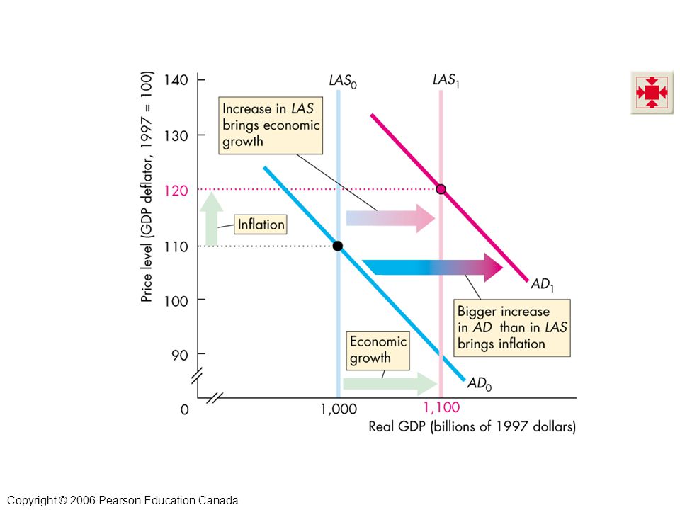
Economic Growth and Inflation Figure illustrates economic growth and inflation.

47
Macroeconomic Equilibrium
Economic growth occurs because the quantity of labour grows, capital is accumulated, and technology advances, all of which increase potential GDP and bring a rightward shift of the LAS curve.

48
Macroeconomic Equilibrium
Inflation occurs because the quantity of money grows faster than potential GDP, which increases aggregate demand by more than long-run aggregate supply. The AD curve shifts rightward faster than the rightward shift of the LAS curve.

50
Macroeconomic Equilibrium
The Business Cycle The business cycle occurs because aggregate demand and the short-run aggregate supply fluctuate, but the money wage does not change rapidly enough to keep real GDP at potential GDP.

51
Macroeconomic Equilibrium
A below full-employment equilibrium is an equilibrium in which potential GDP exceeds real GDP. Figures 21.11(a) and (d) illustrate below full-employment equilibrium. The amount by which potential GDP exceeds real GDP is called a recessionary gap.
 and (d) illustrate below full-employment equilibrium. The amount by which potential GDP exceeds real GDP is called a recessionary gap.")
52
Macroeconomic Equilibrium
A long-run equilibrium is an equilibrium in which potential GDP equals real GDP. Figures 21.11(b) and (d) illustrate long-run equilibrium. In long-run equilibrium, there is full employment.
 and (d) illustrate long-run equilibrium. In long-run equilibrium, there is full employment.")
53
Macroeconomic Equilibrium
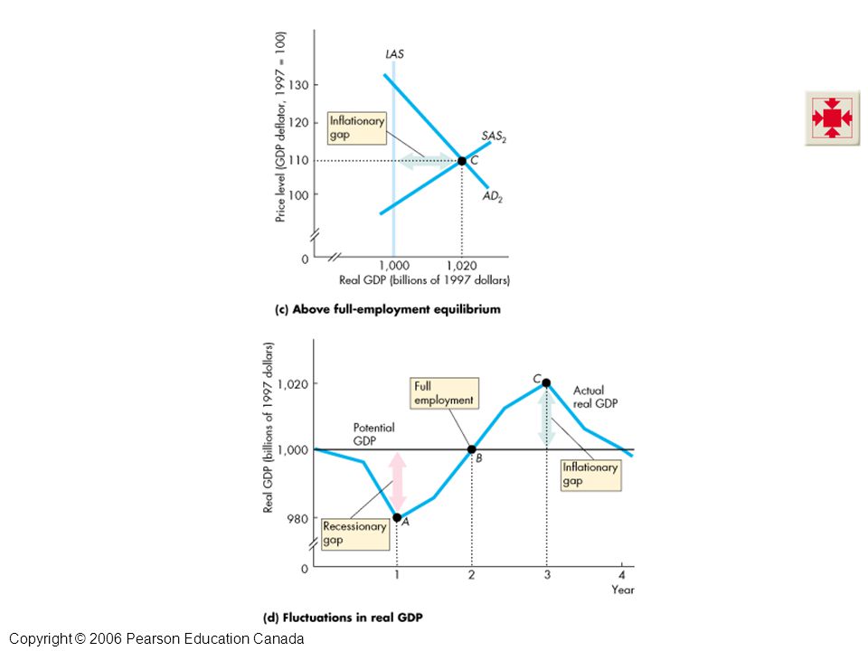
An above full-employment equilibrium is an equilibrium in which real GDP exceeds potential GDP. Figures 21.11(c) and (d) illustrate above full-employment equilibrium. The amount by which real GDP exceeds potential GDP is called an inflationary gap.
 and (d) illustrate above full-employment equilibrium. The amount by which real GDP exceeds potential GDP is called an inflationary gap.")
54
Macroeconomic Equilibrium
Figure 22.11(d) shows how, as the economy moves from one type of short-run equilibrium to another, real GDP fluctuates around potential GDP in a business cycle.
 shows how, as the economy moves from one type of short-run equilibrium to another, real GDP fluctuates around potential GDP in a business cycle.")
56
Macroeconomic Equilibrium
Fluctuations in Aggregate Demand Figure shows the effects of an increase in aggregate demand. Part (a) shows the short-run effects. Starting at long-run equilibrium, an increase in aggregate demand shifts the AD curve rightward.
 shows the short-run effects. Starting at long-run equilibrium, an increase in aggregate demand shifts the AD curve rightward.")
57
Macroeconomic Equilibrium
Firms increase production and rise prices—a movement along the SAS curve.

59
Macroeconomic Equilibrium
Figure 22.12(b) shows the long-run effects. Real GDP increases, the price level rises, and in the new short-run equilibrium, there is an inflationary gap.
 shows the long-run effects. Real GDP increases, the price level rises, and in the new short-run equilibrium, there is an inflationary gap.")
60
Macroeconomic Equilibrium
The money wage rate begins to rise and short-run aggregate supply begins to decrease. The SAS curve gradually shifts leftward. The price level rises and real GDP decreases until it has returned to potential GDP.

62
Macroeconomic Equilibrium
Fluctuations in Aggregate Supply Figure shows the effects of a decrease in aggregate supply. Starting at long-run equilibrium, a rise in the price of oil decreases short-run aggregate supply and the SAS curve shifts leftward.

63
Macroeconomic Equilibrium
Real GDP decreases and the price level rises. The combination of recession and inflation is called stagflation.

65
Canadian Economic Growth, Inflation, and Cycles
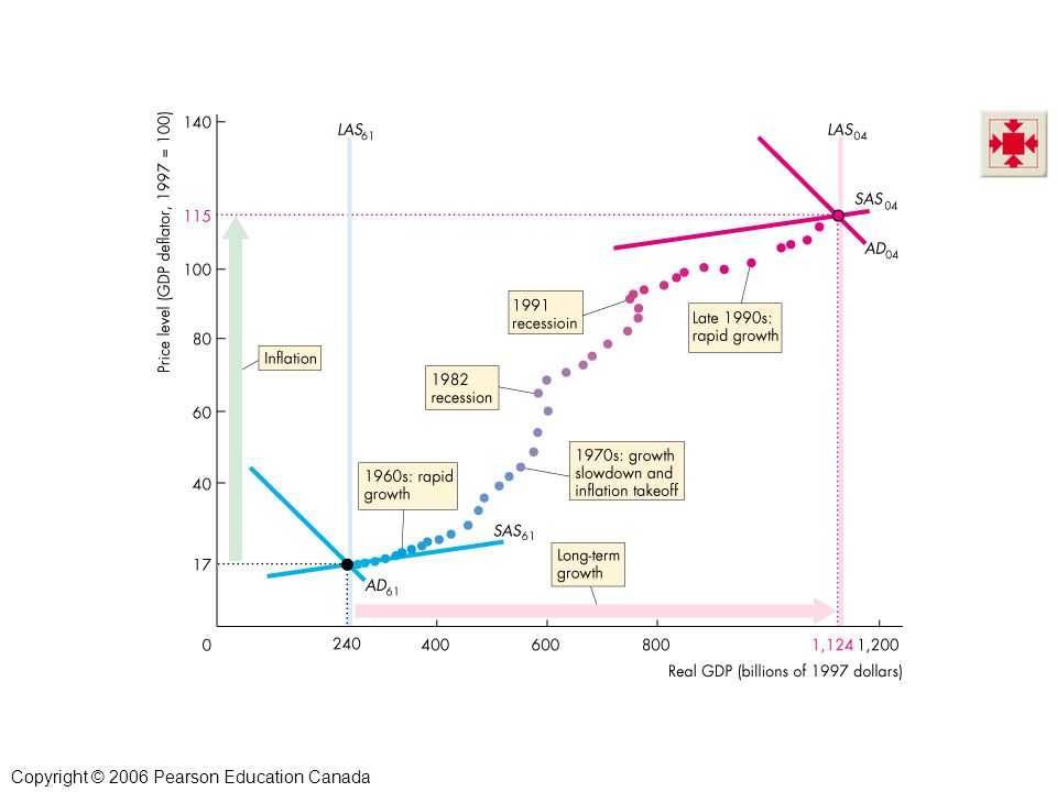
Figure interprets the changes in real GDP and the price level each year from 1961 to 2004 in terms of shifting AD, SAS, and LAS curves. Putting the AS-AD model to work. Don’t neglect the predictions of the model. This is the payoff for the student. With this simple model, we can now say quite a lot about growth, inflation, and the cycle. The price level doesn’t fall, and real GDP rarely falls. The AS-AD model predicts a fall in the price level when either aggregate demand decreases or aggregate supply increases. And the model predicts that real GDP decreases when either aggregate supply or aggregate demand decreases. Students are sometimes bothered by this apparent mismatch between the predictions of the model and the observed economy. The best way to handle this issue is to emphasize that in our actual economy, AS and AD almost always are increasing. When we use the model to simulate the effects of a decrease in either AS or AD, we’re studying what happens relative to the trends in real GDP and the price level. A fall in the price level in the model translates into a lower price level than would otherwise have occurred and a slowing of inflation. The story is similar for real GDP.

66
Canadian Economic Growth, Inflation, and Cycles
The figure shows the business cycle: With rapid growth during the 1960s, slowdown in the 1970s, recessions in 1982 and 1991, and faster growth during the late 1990s …

67
Canadian Economic Growth, Inflation, and Cycles
The figure also shows inflation… …and long-term economic growth.

68
Canadian Economic Growth, Inflation, and Cycles
From1961 to 2004: Real GDP and potential GDP grew from $240 billion to $1,124 billion. The price level rose from 17 to 115. Business cycle expansions alternated with recessions.

70
Canadian Economic Growth, Inflation, and Cycles
Real GDP growth was rapid during the 1960s and late 1990s through 2004 and slower during the 1970s and 1980s. Inflation Inflation was the most rapid during the 1970s. Business Cycles Recessions occurred in 1982 and 1991.

Similar presentations