2. PART 5
ECONOMIC FLUCTUATIONS 14
AS-AD and the Business Cycle
CHAPTER

3. C H A P T E R C H E C K L I S T
When you have completed your study of this chapter, you will be able to
Provide a technical definition of recession and describe the history of the U.S. business cycle. 1
Define and explain the influences on aggregate supply. 2
Economists are ambivalent about the aggregate supply-aggregate demand (AS-AD) model. Real business cycle theorists, who like to build their models from the base of production functions and preferences, don’t use the model because the AS and AD curves are not independent. Technological change shifts both the AS and AD curves simultaneously and in complicated ways. New Keynesian economists have dropped the model in favor of a dynamic variant that places the inflation rate on the y‐axis and the output gap (real GDP minus potential GDP as a percentage of potential GDP) on the x‐axis.
Despite attacks on the model from both sides of the doctrinal spectrum, those of us who spend a good part of our professional lives teaching the principles course recognize the AS-AD model as the key macroeconomic model. For us, the model plays a similar role in the organization of the macroeconomics to that played by the demand and supply model in microeconomics. That is the view taken in this textbook.
The AS-AD model is the best model currently available for introducing students to macroeconomics. It enables them to gain insights into the way the economy works, to organize their study of the subject, and to understand the debates surrounding the effects of policies designed to improve macroeconomic performance.
Define and explain the influences on aggregate demand. 3
Explain how fluctuations in aggregate demand and aggregate supply create the business cycle. 4

4. 14.1 BUSINESS-CYCLE DEFINITIONS AND FACTS
The business cycle is a periodic but irregular up-and-down movement in production and jobs.
A business cycle has two phases, expansion and recession, and two turning point, a peak and a trough.
Dating Business-Cycle Turning Points
The task of identifying and dating business-cycle phases and turning points is performed by a private research organization, the National Bureau of Economic Research (NBER).

5. 14.1 BUSINESS-CYCLE DEFINITIONS AND FACTS
To date the business-cycle turning points, the NBER needs a definition of recession.
Recession
A decrease in real GDP that lasts for at least two quarters (six months) or a period of significant decline in total output, income, employment, and trade, usually lasting from six months to a year and marked by widespread contractions in many sectors of the economy.

6. 14.1 BUSINESS-CYCLE DEFINITIONS AND FACTS
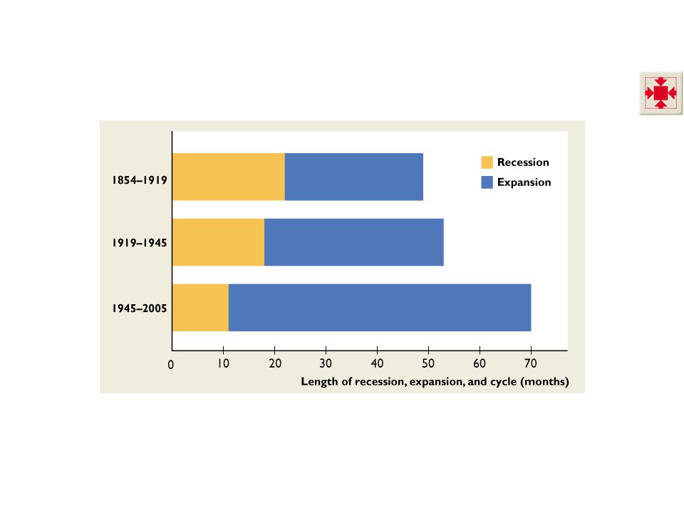
U.S. Business-Cycle History
The NBER has identified 33 complete cycles starting from a trough in December 1854.
Over all 33 complete cycles:
The average length of an expansion is 35 months and the average length of a recession is 18 months.
The average time from trough to trough is 53 months.

7. 14.1 BUSINESS-CYCLE DEFINITIONS AND FACTS
So over the 152 years since 1854, the U.S. economy has been in:
Recession for about one third of the time
Expansion for about two thirds of the time.
The 152-year averages hide significant changes that have occurred in the length of a cycle and the relative length of the recession and expansion phases.

8. 14.1 BUSINESS-CYCLE DEFINITIONS AND FACTS
Figure 14.1 summarizes U.S. recession, expansion, and cycle length since 1854.
Recessions have shortened.
Expansions have lengthened, and complete cycles have lengthened.

10. 14.1 BUSINESS-CYCLE DEFINITIONS AND FACTS
Recent Cycles
The last completed cycle began at a trough of March 1991 and ended at a trough of November 2001.
The economy expanded from March 1991 until March 2001.
This expansion, which lasted for 120 months, was the longest in U.S. history.

11. 14.1 BUSINESS-CYCLE DEFINITIONS AND FACTS
Figure 14.2(a) shows the recent cycles in real GDP.
Recessions began in mid-1990 and in first quarter of 2001.
The longest expansion in U.S. history ran from the March 1991 to March 2001.

12. 14.1 BUSINESS-CYCLE DEFINITIONS AND FACTS
When real GDP decreased in the recession (part a),
The unemployment rate increased (part b).
And a little later, the inflation rate decreased (part c).
As real GDP increased back toward potential GDP, the unemployment rate fell toward the natural unemployment rate and the inflation rate fell.

14. 14.2 AGGREGATE SUPPLY Real GDP depends on the quantities of
Labor employed
Capital, human capital, and the state of technology
Land and natural resources
Entrepreneurial talent

15. 14.2 AGGREGATE SUPPLY At full employment:
The real wage rate makes the quantity of labor demanded equal to the quantity of labor supplied.
Real GDP equals potential GDP.
Over the business cycle:
The quantity of labor employed fluctuates around its full employment level.
Real GDP fluctuates around potential GDP.

16. Aggregate Supply Basics
Aggregate supply is the relationship between the quantity of real GDP supplied and the price level when all other influences on production plans remain the same.
Other things remaining the same,
When the price level rises, the quantity of real GDP supplied increases.
When the price level falls, the quantity of real GDP supplied decreases.

17. 14.2 AGGREGATE SUPPLY
Along the aggregate supply curve, the only influence on production plans that changes is the price level.
All the other influences on production plans remain constant. Among these other influences are
The money wage rate
The money prices of other resources
In contrast, along the potential GDP line, when the price level changes the money wage rate changes to keep the real wage rate at the full-employment level.

18. 14.2 AGGREGATE SUPPLY
Figure 14.3 shows the aggregate supply schedule and aggregate supply curve.
Each point A to E on the AS curve corresponds to a row of the schedule.
It’s difficult to start using the AS-AD model until you are convinced that students have bought into the notion that the aggregate supply curve is upward sloping and the reasons behind it. The AS curve that is used in this chapter is a short-run aggregate supply curve because it assumes that product prices and resources prices do not move in lock step with one another. That is to say that wages, materials prices, energy prices and the like move with a lag behind product prices. To launch your lecture, walk through this thought experiment with your students. Ask your class if firms are likely to be motivated to step up production in the face of rising product prices. They will have no trouble responding in the affirmative. Now tell your students that the higher price is actually the result of an increase in the general price level. Ask them how quickly workers are likely to respond by asking for wage increases. The answer is that it will take time for workers to see that the general price level has risen and that their real wages are now lower. Eventually they will demand higher wages. Firms will grant the wage increase in the face of higher profits. But until workers realize that their real wage has fallen, firms are in the position of receiving higher prices with no change in money wages so they increase their production. And with this result, you have demonstrated the upward-sloping aggregate supply curve!

19. 14.2 AGGREGATE SUPPLY
1. Potential GDP is $10 trillion and when the price level is 110, real GDP equals potential GDP.
2. If the price level is above 110, real GDP exceeds potential GDP.
3. If the price level is below 110, real GDP exceeds potential GDP.

21. 14.2 AGGREGATE SUPPLY Why the AS Curve Slopes Upward
When the price level rises and the money wage rate is constant, the real wage rate falls and employment increases. The quantity of real GDP supplied increases.
When the price level falls and the money wage rate is constant, the real wage rate rises and employment decreases. The quantity of real GDP supplied decreases.

22. Changes in Aggregate Supply
Aggregate supply changes when any influence on production plans other than the price level changes.
In particular, aggregate supply changes when
Potential GDP changes.
The money wage rate changes.
The money prices of other resources change.

23. 14.2 AGGREGATE SUPPLY Changes in Potential GDP
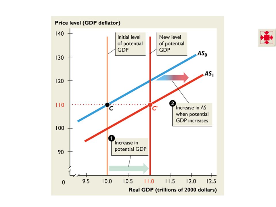
Anything that changes potential GDP changes aggregate supply and shifts the aggregate supply curve.
Figure 14.4 on the next slide illustrates.

24. 14.2 AGGREGATE SUPPLY
Point C at the intersection of the potential GDP line and AS curve is an anchor point.
1. An increase in potential GDP shifts the potential GDP line rightward and ...
2. The aggregate supply curve shifts rightward from AS0 to AS1.

26. 14.2 AGGREGATE SUPPLY Changes in Money Wages and Other Resource Prices
A change in the money wage rate or the money price of another resource changes aggregate supply because it changes firms’ costs.
The higher the money wage rate, the higher are firms’ costs and the smaller is the quantity that firms are willing to supply at each price level.
So an increase in the money wage rate decreases aggregate supply.

27. 14.2 AGGREGATE SUPPLY
Figure 14.5 shows the effect of a change in the money wage rate.
A rise in the money wage rate decreases aggregate supply and the aggregate supply curve shifts leftward from AS0 to AS2.
A rise in the money wage rate does not change potential GDP.

29. 14.3 AGGREGATE DEMAND
The quantity of real GDP demanded is the total amount of final goods and services produced in the United States that people, businesses, governments, and foreigners plan to buy.
This quantity is the sum of the real consumption expenditure (C), investment (I), government expenditure on goods and services (G), and exports (X) minus imports (M).
That is,
Y = C + I + G + X – M

30. Aggregate Demand Basics
Aggregate demand is the relationship between the quantity of real GDP demanded and the price level when all other influences on expenditure plans remain the same.
Other things remaining the same,
When the price level rises, the quantity of real GDP demanded decreases.
When the price level falls, the quantity of real GDP demanded increases.

31. 14.3 AGGREGATE DEMAND
Figure 14.6 shows the aggregate demand schedule and aggregate demand curve.
Each point A to E on the AD curve corresponds to a row of the schedule.

32. 14.3 AGGREGATE DEMAND The quantity of real GDP demanded
1. Decreases when the price level rises.
2. Increases when the price level falls.

34. 14.3 AGGREGATE DEMAND
The price level influences the quantity of real GDP demanded because a change in the price level brings changes in
The buying power of money
The real interest rate
The real prices of exports and imports

35. 14.3 AGGREGATE DEMAND The Buying Power of Money
A rise in the price level lowers the buying power of money and decreases the quantity of real GDP demanded.
For example, if the price level rises and other things remain the same, a given quantity of money will buy less goods and services, so people cut their spending.
So the quantity of real GDP demanded decreases.

36. 14.3 AGGREGATE DEMAND The Real Interest Rate
When the price level rises, the real interest rate rises.
An increase in the price level increases the amount of money that people want to hold—increases the demand for money.
When the demand for money increases, the nominal interest rate rises.
In the short run, the inflation rate doesn’t change, so a rise in the nominal interest rate brings a rise in the real interest rate.

37. 14.3 AGGREGATE DEMAND
Faced with a higher real interest rate, businesses and people delay plans to buy new capital goods and consumer durable goods and cut back on spending.
So the quantity of real GDP demanded decreases.

38. 14.3 AGGREGATE DEMAND The Real Prices of Exports and Imports
When the U.S. price level rises and other things remain the same, the prices in other countries do not change.
So a rise in the U.S. price level makes U.S.-made goods and services more expensive relative to foreign-made goods and services.
This change in real prices encourages people to spend less on U.S.-made items and more on foreign-made items.

39. 14.3 AGGREGATE DEMAND
In the long run, when the price level changes by more in one country than in other countries, the exchange rate changes.
The exchange rate neutralizes the price level change, so this international price effect on buying plans is a short-run effect only.
But the short-run effect is powerful.

40. Changes in Aggregate Demand
A change in any factor that influences expenditure plans other than the price level brings a change in aggregate demand.
When aggregate demand increases, the aggregate demand curve shifts rightward.
When aggregate demand decreases, the aggregate demand curve shifts leftward.
Some of the same issues regarding change in demand and change in quantity demanded not only apply in the microeconomic model but also apply to the aggregate supply and aggregate demand curves as well. Remind your students that a change in the price level does not shift the aggregate supply curve or aggregate demand curve. A change in the price level results in movements along the curves. You can also involve your students in the material by asking them a few hypothetical questions. Ask your class what will happen to the aggregate demand curve in each of the following cases:
a. A cut in taxes.
b. An increase in expected future profit.
c. A cut in government spending.
d. An increase in foreign income.
e. A rise in the price level abroad.
Each of these examples gives students practice shifting the aggregate demand curve rightward and leftward as well as understanding why it shifts in the direction that it does.

41. 14.3 AGGREGATE DEMAND The factors that change aggregate demand are
Expectations about the future
Fiscal policy and monetary policy
The state of the world economy

42. 14.3 AGGREGATE DEMAND Expectations
An increase in expected future income increases the amount of consumption goods that people plan to buy today and increases aggregate demand.
An increase in expected future inflation increases aggregate demand today because people decide to buy more goods and services now before their prices rise.
An increase in expected future profit increases the investment that firms plan to undertake today and increases aggregate demand.

43. 14.3 AGGREGATE DEMAND Fiscal Policy and Monetary Policy
Government can influence aggregate demand by set-ting and changing taxes, transfer payments, and government expenditure on goods and services.
The Federal Reserve can influence aggregate demand by changing the quantity of money and the interest rate.

44. 14.3 AGGREGATE DEMAND
A tax cut or an increase in either transfer payments or government expenditure on goods and services increases aggregate demand.
A cut in the interest rate or an increase in the quantity of money increases aggregate demand.

45. 14.3 AGGREGATE DEMAND The World Economy
The foreign exchange rate and foreign income influence aggregate demand.
Foreign exchange rate is the amount of foreign currency you can buy with a U.S. dollar.
Other things remaining the same, a rise in the foreign exchange rate decreases aggregate demand.
An increase in foreign income increases U.S. exports and increases U.S. aggregate demand.

46. 14.3 AGGREGATE DEMAND Figure 14.7 shows changes in aggregate demand.
1. Aggregate demand increases if
Expected future income, inflation, or profits increase.
Fiscal policy or monetary policy increase planned expenditure.
The exchange rate falls or foreign income increases.

47. 14.3 AGGREGATE DEMAND 2. Aggregate demand decreases if:
Expected future income, inflation, or profits decrease.
Fiscal policy or monetary policy decrease planned expenditure.
The exchange rate rises or foreign income decreases.

49. The Aggregate Demand Multiplier
The aggregate demand multiplier is an effect that magnifies changes in expenditure plans and brings potentially large fluctuations in aggregate demand.
When any influence on aggregate demand changes expenditure plans:
The change in expenditure changes income.
And the change in income induces a change in consumption expenditure.

50. 14.3 AGGREGATE DEMAND
The increase in aggregate demand is the initial increase in expenditure plus the induced increase in consumption expenditure.

51. 14.3 AGGREGATE DEMAND
Figure 14.8 shows the aggregate demand multiplier.
1. An increase in investment increases aggregate demand and increases income.
2..The increase in income induces an increase in consumption expenditure, so
3. Aggregate demand increases by more than the initial increase in investment.

53. 14.4 UNDERSTANDING BUSINESS CYCLES
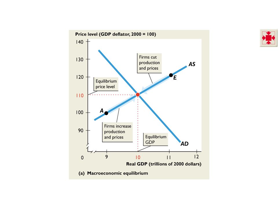
Aggregate supply and aggregate demand determine real GDP and the price level.
Macroeconomic equilibrium occurs when the quantity of real GDP demanded equals the quantity of real GDP supplied at the point of intersection of the AD curve and the AS curve.
Figure 14.9(a) on the next slide illustrates macroeconomic equilibrium.

54. 14.4 UNDERSTANDING BUSINESS CYCLES
Suppose that the price level is 120 and that real GDP is $11 trillion, at point E.
The quantity of real GDP demand is less than $11 trillion and firms cannot sell all they produce, so they cut production and lower prices.

55. 14.4 UNDERSTANDING BUSINESS CYCLES
Suppose that the price level is 100 and that real GDP is $9 trillion, at point A.
The quantity of real GDP demand exceeds $9 trillion and firms cannot meet the demand for their output, so they increase production and raise prices.

56. 14.4 UNDERSTANDING BUSINESS CYCLES
Macroeconomic equilibrium occurs when the price level is 110 and real GDP is $10 trillion.

58. 14.4 UNDERSTANDING BUSINESS CYCLES
Three possible macroeconomic equilibriums are
1. Below full-employment equilibrium, when potential GDP exceeds equilibrium real GDP.
2. Full-employment equilibrium, when equilibrium real GDP equal potential GDP.
3. Above full-employment equilibrium, when equilibrium real GDP exceeds potential GDP.

60. 14.4 UNDERSTANDING BUSINESS CYCLES
Aggregate Demand Fluctuations
Fluctuations in aggregate demand are one of the sources of the business cycle.
To focus on the business cycle, we’ll ignore economic growth and inflation and suppose that potential GDP and the full-employment price level is constant.
Figure in the next slide illustrates the business cycle.
Don’t neglect the predictions of the model. This is the payoff for the student. With this simple model, we can now say quite a lot about growth, inflation, and the business cycle. However, when you do so, be aware that the AS-AD model predicts a fall in the price level when either aggregate demand decreases or aggregate supply increases. And the model predicts that real GDP decreases when either aggregate supply or aggregate demand decreases. But, some students object by pointing out that GDP rarely decreases and the price level rarely falls. These students are bothered by this apparent mismatch between the predictions of the model and the observed economy. The best way to handle this issue is to emphasize that in our actual economy, aggregate supply and aggregate demand almost always are increasing. When we use the model to simulate the effects of a decrease in either aggregate supply and aggregate demand, we’re studying what happens relative to the trends in real GDP and the price level. A fall in the price level in the model translates into a lower price level than would otherwise have occurred and a slowing of inflation. The story is similar for real GDP.

61. 14.4 UNDERSTANDING BUSINESS CYCLES
Fluctuations in aggregate demand bring fluctuations in actual real GDP around potential GDP.
In year 1, real GDP equals potential GDP. The economy is at full employment.

62. 14.4 UNDERSTANDING BUSINESS CYCLES
In year 2, at a business cycle peak, real GDP exceeds potential GDP. The economy is operating at above full employment.
In year 3, real GDP equals potential GDP. The economy is back at full employment.

63. 14.4 UNDERSTANDING BUSINESS CYCLES
In year 4, at a business cycle trough, real GDP is below potential GDP. The economy is operating at below full employment.
In year 5, real GDP equals potential GDP. The economy is back at full employment.

65. 14.4 UNDERSTANDING BUSINESS CYCLES
Aggregate Supply Fluctuations
Aggregate supply fluctuates for two types of reasons:
Potential GDP grows at an uneven pace.
The money price of a major resource, such as crude oil, might change.
Stagflation
A combination of recession (falling real GDP) and inflation (rising price level).

66. 14.4 UNDERSTANDING BUSINESS CYCLES
Figure shows an oil price cycle.
A rise in the price of oil decreases aggregate supply and shifts the AS curve leftward to AS1.
Real GDP decreases, and the price level rises.
The economy experiences stagflation.

68. 14.4 UNDERSTANDING BUSINESS CYCLES
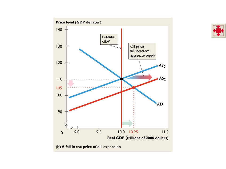
A fall in the price of oil increases aggregate supply and shifts the AS curve rightward to AS2.
The price level falls and real GDP increases.
The economy experiences an expansion.

70. 14.4 UNDERSTANDING BUSINESS CYCLES
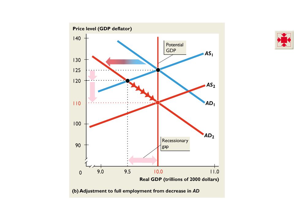
Adjustment Toward Full Employment
When the economy is away from full employment, forces operate to restore full employment.
Inflationary gap
A gap that exists when real GDP exceeds potential GDP and that brings a rising price level.
Recessionary gap
A gap that exists when potential GDP exceeds real GDP and that brings a falling price level.
Reinforce the movement toward long-run equilibrium with a curve-shifting exercise. Take the case where the AD curve shifts rightward. The fact that the initial equilibrium occurs where the new AD curve intersects the AS curve is not difficult. But the notion that the AS curve shifts leftward as time passes is difficult for many students. The trick to making this idea clear is to spend enough time when initially discussing the AS curve so that the students realize that wages and other input prices remain constant along an AS curve. Once the students see this point, they can understand that, as input prices increase in response to the higher level of prices, the AS curve shifts leftward. Avoid confusing students by using ‘up’ to correspond to a decrease in aggregate supply. But do point out that that when the AS curve shifts leftward it is moving vertically upward, as input prices rise to become consistent with potential GDP and the new long-run equilibrium price level. Most students find it easier to see why the AS curve shifts leftward once they see that rising input prices shift the curve vertically upward

71. 14.4 UNDERSTANDING BUSINESS CYCLES
Figure shows adjustments toward full employment.
Real GDP exceeds potential GDP — there is an inflationary gap —and the price level rises.
As the money wage rate gradually rises, aggregate supply decreases, real GDP decreases, and the price level rises farther.

73. 14.4 UNDERSTANDING BUSINESS CYCLES
Potential GDP exceeds real GDP—recessionary gap— and the price level falls.
Eventually, the money wage rate starts to fall, aggregate supply increases, real GDP increases, and the price level falls farther.

75. AS-AD in YOUR Life Consider the U.S. economy right now.
Using the knowledge you have accumulated over the course and information you have read in the current news, do you think real GDP is currently above, below, or at potential GDP?
Talk to your class mates about where they see the U.S. economy right now. Is there a consensus?
What are the main pressures on AS and AD right now?
Do you think that real GDP will expand more quickly or more slowly over the coming months?
Will the gap between real GDP and potential GDP widen or narrow?