1. University of Waterloo
Department of Mechanical Engineering
ME Mechanical Design 1
Partial notes – Part 4 (Fatigue)
(G. Glinka)
Fall 2005

2. FATIGUE - What is it? Ni = ? Np = ? NT = ?
Metal Fatigue is a process which causes premature irreversible damage or failure of a component subjected to repeated loading.

3. Metallic Fatigue
A sequence of several, very complex phenomena encompassing several disciplines:
motion of dislocations
surface phenomena
fracture mechanics
stress analysis
probability and statistics
Begins as an consequence of reversed plastic deformation within a single crystallite but ultimately may cause the destruction of the entire component
Influenced by a component’s environment
Takes many forms:
fatigue at notches
rolling contact fatigue
fretting fatigue
corrosion fatigue
creep-fatigue
Fatigue is not cause of failure per se but leads to the final fracture event.

4. The Broad Field of Fracture Mechanics
(from Ewalds & Wanhil, ref.3)

5. Intrusions and Extrusions: The Early Stages of Fatigue Crack Formation

6. Schematic of Fatigue Crack Initiation Subsequent Growth Corresponding and Transition From Mode II to Mode I c Δσ
Locally, the crack grows in shear;
macroscopically it grows in tension.

7. The Process of Fatigue The Materials Science Perspective: Cyclic slip,
Fatigue crack initiation,
Stage I fatigue crack growth,
Stage II fatigue crack growth,
Brittle fracture or ductile rupture

8. Features of the Fatigue Fracture Surface of a Typical Ductile Metal Subjected to Variable Amplitude Cyclic Loading
A – fatigue crack area
B – area of the final static failure
(Collins, ref. 22 )

9. Appearance of Failure Surfaces Caused by Various Modes of Loading (SAE Handbook)

10. Factors Influencing Fatigue Life
Applied Stresses
Stress range – The basic cause of plastic deformation and consequently the accumulation of damage
Mean stress – Tensile mean and residual stresses aid to the formation and growth of fatigue cracks
Stress gradients – Bending is a more favorable loading mode than axial loading because in bending fatigue cracks propagate into the region of lower stresses
Materials
Tensile and yield strength – Higher strength materials resist plastic deformation and hence have a higher fatigue strength at long lives. Most ductile materials perform better at short lives
Quality of material – Metallurgical defects such as inclusions, seams, internal tears, and segregated elements can initiate fatigue cracks
Temperature – Temperature usually changes the yield and tensile strength resulting in the change of fatigue resistance (high temperature decreases fatigue resistance)
Frequency (rate of straining) – At high frequencies, the metal component may be self-heated.

11. Strength-Fatigue Analysis Procedure
Component
Geometry
Loading
History
Stress-Strain
Analysis
Damage
Allowable Load - Fatigue Life
Material
Properties
Information path in strength and fatigue life prediction procedures

12. Stress Parameters Used in Static Strength and Fatigue Analysesdn T r
speak
Stress S b) n y dn T r
speak
Stress M S

13. Constant and Variable Amplitude Stress Histories; Definition of a Stress Cycle & Stress Reversal
One cycle m
max
min
Stress
Time
Constant amplitude stress history a)
Variable amplitude stress history
One reversal b)
In the case of the peak stress history the important parameters are:

14. Stress History and the “Rainflow” Counted Cycles
Time
Stress history
Rainflow counted cycles
i-1
i-2
i+1 i
i+2
A rainflow counted cycle is identified when any two adjacent reversals in thee stress history satisfy the following relation:

15. The Mathematics of the Cycle Rainflow Counting Method for Fatigue Analysis of Stress/Load Histories
A rainflow counted cycle is identified when any two adjacent reversals in thee stress history satisfy the following relation:
The stress amplitude of such a cycle is:
The stress range of such a cycle is:
The mean stress of such a cycle is:

17. Stress History Stress (MPa)x10 Reversal point No. -3 -2 -1 1 2 3 4 5 61 2 3 4 5 6 7 8 9 10 11 12 13 14
Stress (MPa)x10
Reversal point No.

18. Stress History Stress (MPa)x10 Reversal point No. -3 -2 -1 1 2 3 4 5 61 2 3 4 5 6 7 8 9 10 11 12 13 14
Stress (MPa)x10
Reversal point No.

19. Stress History Stress (MPa)x10 Reversal point No. -3 -2 -1 1 2 3 4 5 61 2 3 4 5 6 7 8 9 10 11 12 13 14
Stress (MPa)x10
Reversal point No.

20. Stress History Stress (MPa)x10 Reversal point No. -3 -2 -1 1 2 3 4 5 61 2 3 4 5 6 7 8 9 10 11 12 13 14
Stress (MPa)x10
Reversal point No.

21. Number of Cycles According to the Rainflow Counting Procedure (N
Number of Cycles According to the Rainflow Counting Procedure (N. Dowling, ref. 2)

22. The Fatigue S-N method (Nominal Stress Approach)
The principles of the S-N approach (the nominal stress method)
Fatigue damage accumulation
Significance of geometry (notches) and stress analysis in fatigue evaluations of engineering structures
Fatigue life prediction in the design process

23. Wöhler’s Fatigue Test A B
Note! In the case of smooth components such as the railway axle the nominal stress and the local peak stress are the same!
Smin
Smax

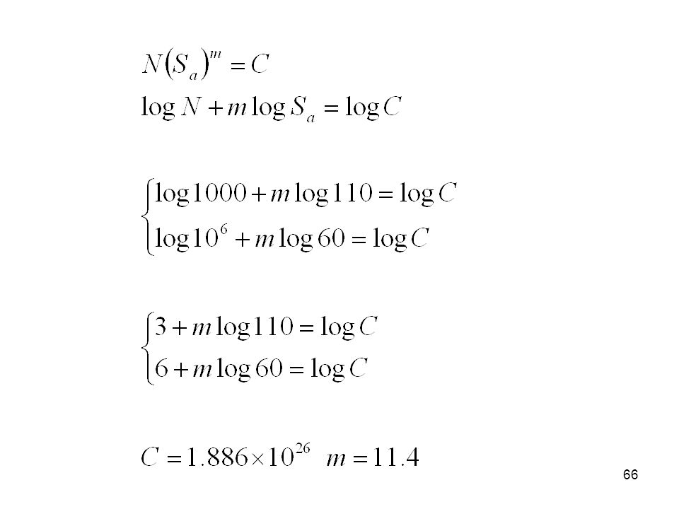
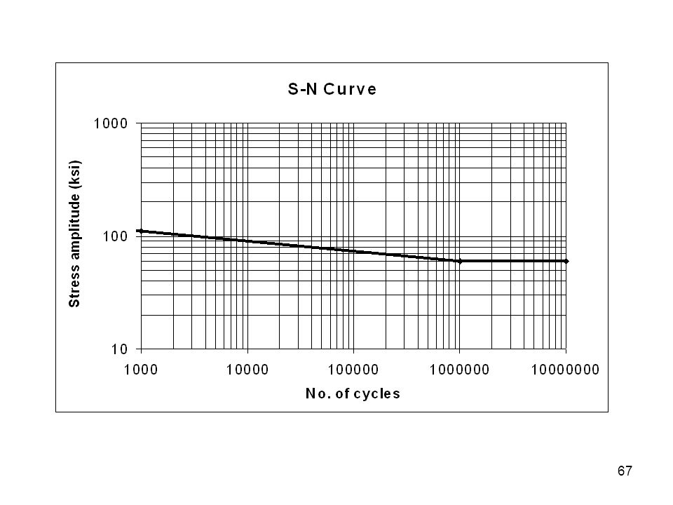
24. Characteristic parameters of the S - N curve are:
Se - fatigue limit corresponding to N = 1 or 2106 cycles for
steels and N = 108 cycles for aluminum alloys,
S103 - fully reversed stress amplitude corresponding to N = 103
cycles
m - slope of the high cycle regime curve (Part 2)
Fully reversed axial S-N curve for AISI 4130 steel. Note the break at the LCF/HCF transition and the endurance limit
Number of cycles, N
Stress amplitude, Sa (ksi) Sy Se
Part 1
Part 2
Part 3
Infinite life Su
S103
Fatigue S-N curve

25. S103 = 0.90Su and Se = S106 = 0.5 Su - bending
Most of available S - N fatigue data has been obtained from fully reversed rotational bending tests. However, material behavior and the resultant S - N curves are different for different types of loading. It concerns in particular the fatigue limit Se.
The stress endurance limit, Se, of steels (at 106 cycles) and the fatigue strength, S103 corresponding to 103 cycles for three types of loading can be approximated as (ref. 1, 23, 24):
S103 = 0.90Su and Se = S106 = 0.5 Su bending
S103 = 0.75Su and Se = S106 = Su - axial
S103 = 0.72Su and Se = S106 = 0.29 Su torsion
103
104
105
106
107
0.1
0.3
0.5
1.0
S103 Se
Number of cycles, Log(N)
Relative stress amplitude, Sa/Su
Torsion
Axial
Bending

26. Approximate endurance limit for various materials:
Magnesium alloys (at 108 cycles) Se = 0.35Su
Copper alloys (at 108 cycles) Su< Se <0.50Su
Nickel alloys (at 108 cycles) Su <Se < 0.50Su
Titanium alloys (at 107 cycles) Su <Se< 0.65Su
Al alloys (at 5x108 cycles) Se = 0.45Su (if Su ≤ 48 ksi) or Se = 19 ksi (if Su> 48 ksi)
Steels (at 106 cycles) Se = 0.5Su (if Su ≤ 200 ksi) or Se = 100 ksi (if Su>200 ksi)
Irons (at 106 cycles) Se = 0.4Su (if Su ≤ 60 ksi) or Se = 24 ksi (if Su> 60 ksi)
S – N curve

27. Fatigue Limit – Modifying Factors Fatigue limit of a machine part, Se
For many years the emphasis of most fatigue testing was to gain an empirical understanding of the effects of various factors on the base-line S-N curves for ferrous alloys in the intermediate to long life ranges. The variables investigated include:
- Rotational bending fatigue limit, Se’,
- Surface conditions, ka,
- Size, kb,
- Mode of loading, kc, Se = ka kb kc kd ke kf·Se’
- Temperature, kd
- Reliability factor, ke
- Miscellaneous effects (notch), kf
Fatigue limit of a machine part, Se

28. Surface Finish Effects on Fatigue Endurance LimitCa
Effect of various surface finishes on the fatigue limit of steel. Shown are values of the ka, the ratio of the fatigue limit to that for polished specimens.
Below a generalized empirical graph is shown which can be used to estimate the effect of surface finish in comparison with mirror-polished specimens [Shigley (23), Juvinal (24), Bannantine (1) and other textbooks].
Surface Finish Effects on Fatigue Endurance Limit
The scratches, pits and machining marks on the surface of a material add stress concentrations to the ones already present due to component geometry. The correction factor for surface finish is sometimes presented on graphs that use a qualitative description of surface finish such as “polished” or “machined”.
(from J. Bannantine, ref.1) ka

29. Size Effects on Endurance Limit
Fatigue is controlled by the weakest link of the material, with the probability of existence (or density) of a weak link increasing with material volume. The size effect has been correlated with the thin layer of surface material subjected to 95% or more of the maximum surface stress.
There are many empirical fits to the size effect data. A fairly conservative one is:
The size effect is seen mainly at very long lives.
The effect is small in diameters up to 2.0 in (even in bending and torsion).
Stress effects in non-circular cross section members
In the case of non-circular members the approach is based on so called effective diameter, de.
The effective diameter, de, for non-circular cross sections is obtained by equating the volume of material stressed at and above 95% of the maximum stress to the same volume in the rotating-bending specimen.

30. + -
0.95max
max
0.05d/2
0.95d
The effective diameter, de, for members with non-circular cross sections
The material volume subjected to stresses   0.95max is concentrated in the ring of 0.05d/2 thick.
The surface area of such a ring is:
* rectangular cross section under bending F
0.95t t
Equivalent diameter

31. Loading Effects on Endurance Limit
The ratio of endurance limits for a material found using axial and rotating bending tests ranges from 0.6 to 0.9.
The ratio of endurance limits found using torsion and rotating bending tests ranges from 0.5 to 0.6. A theoretical value obtained from von Mises-Huber-Hencky failure criterion is been used as the most popular estimate.

32. Temperature Effect
From: Shigley and Mischke, Mechanical Engineering Design, 2001

33. Reliability factor ke
The reliability factor accounts for the scatter of reference data such as the rotational bending fatigue limit Se’.
The estimation of the reliability factor is based on the assumption that the scatter can be approximated by the normal statistical probability density distribution.
The values of parameter za associated with various levels of reliability can be found in Table 7-7 in the textbook by Shigley et.al.

34. S-N curves for assigned probability of failure; P - S - N curves
(source: S. Nishijima, ref. 39)
S-N curves for assigned probability of failure; P - S - N curves

35. Stress concentration factor, Kt, and the notch factor effect, kf
Fatigue notch factor effect kf depends on the stress concentration factor Kt (geometry), scale and material properties and it is expressed in terms of the Fatigue Notch Factor Kf.

36. Stresses in axisymmetric notched body1
speak sn
s22
s11
s33 3 2 A D B C F
A, B
Stresses in axisymmetric notched body

37. Stresses in prismatic notched body
A, B, C
s22
s33 D E
s11
s peak sn 3 2 A B C F 1

38. Stress concentration factors used in fatigue analysis
n, S x dn W r
s peak
Stress S n M

39. Stress concentration factors, Kt, in shafts
Bending load
Axial load
S =

40. S =

41. Similarities and differences between the stress field near the notch and in a smooth specimenx dn W r
peak
Stress S
n=S
peak= n=S P

42. The Notch Effect in Terms of the Nominal Stressnp n1
DS2
cycles N0 N2
Sesmooth
N (DS)m = C
DSmax
Stress range S n2 n3 n4
Fatigue notch factor!

43. Definition of the fatigue notch factor Kf1 2 3
Nsmooth
speak
Stress
Nnotched M
Definition of the fatigue notch factor Kf
s22= speak S Se

44. PETERSON's approach a – constant, NEUBER’s approach
r – notch tip radius;
NEUBER’s approach
ρ – constant,
r – notch tip radius

45. The Neuber constant ‘ρ’ for steels and aluminium alloys

46. Curves of notch sensitivity index ‘q’ versus notch radius (McGraw Hill Book Co, from ref. 1)

47. Illustration of the notch/scale effect
Plate 1
W1 = 5.0 in
d1 = 0.5 in.
Su = 100 ksi
Kt = 2.7
q = 0.97
Kf1 = 2.65
Illustration of the notch/scale effect
Plate 2
W2= 0.5 in
d2 = 0.5 i
q = 0.78
Kf1 = 2.32
peak
m1  d1 W1 d2 W2
m2

48. Procedures for construction of approximate fully reversed S-N curves for smooth and notched components
Nf (logartmic)
Juvinal/Shigley method
Collins method
Sar, ar – nominal/local stress amplitude at zero mean stress m=0 (fully reversed cycle)!
f’

49. Procedures for construction of approximate fully reversed S-N curves for smooth and notched components
Sar, ar – nominal/local stress amplitude at zero mean stress m=0 (fully reversed cycle)!
Sar (logartmic)
Nf (logartmic)
Manson method
0.9Su
100
101
102
103
104
105
106
2·106
Se’kakckbkdke
Se’kakckbkdkekf Se

50. NOTE!
The empirical relationships concerning the S –N curve data are only estimates! Depending on the acceptable level of uncertainty in the fatigue design, actual test data may be necessary.
The most useful concept of the S - N method is the endurance limit, which is used in “infinite-life”, or “safe stress” design philosophy.
In general, the S – N approach should not be used to estimate lives below 1000 cycles (N < 1000).

51. Constant amplitude cyclic stress histories
Fully reversed
m = 0, R = -1
Pulsating
m = a R = 0
Cyclic
m > 0 R > 0

52. Mean Stress Effect time Stress amplitude, Sa sm> 0 sm= 0 sm< 0
sm< 0
sm= 0
sm> 0
No. of cycles, logN
2*106
Stress amplitude, logSa

53. Steel AISI 4340, Sy = 147 ksi (Collins)
The tensile mean stress is in general detrimental while the compressive mean stress is beneficial or has negligible effect on the fatigue durability.
Because most of the S – N data used in analyses was produced under zero mean stress (R = -1) therefore it is necessary to translate cycles with non- zero mean stress into equivalent cycles with zero mean stress producing the same fatigue life.
There are several empirical methods used in practice:
The Hiagh diagram was one of the first concepts where the mean stress effect could be accounted for. The procedure is based on a family of Sa – Sm curves obtained for various fatigue lives.
Steel AISI 4340,
Sy = 147 ksi (Collins)

54. Mean Stress Correction for Endurance Limit
Gereber (1874)
Goodman (1899)
Soderberg (1930)
Morrow (1960)
Sa – stress amplitude applied at the mean stress Sm≠ 0 and fatigue life N = 1-2x106cycles.
Sm- mean stress
Se- fatigue limit at Sm=0
Su- ultimate strength
f’- true stress at fracture

55. Mean stress correction for arbitrary stress amplitude applied at non-zero mean stress
Gereber (1874)
Goodman (1899)
Soderberg (1930)
Morrow (1960)
Sa – stress amplitude applied at the mean stress Sm≠ 0 and resulting in fatigue life of N cycles.
Sm- mean stress
Sar- fully reversed stress amplitude applied at mean stress Sm=0 and resulting in the same fatigue life of N cycles
Su- ultimate strength
f’- true stress at fracture

56. Comparison of various methods of accounting for the mean stress effect
Most of the experimental data lies between the Goodman and the yield line!

57. Approximate Goodman’s diagrams for ductile and brittle materialsKf

58. The following generalisations can be made when discussing mean stress effects:
1. The Söderberg method is very conservative and seldom used.
3. Actual test data tend to fall between the Goodman and Gerber curves.
3. For hard steels (i.e., brittle), where the ultimate strength approaches the true fracture stress, the Morrow and Goodman lines are essentially the same. For ductile steels (of > S,,) the Morrow line predicts less sensitivity to mean stress.
4. For most fatigue design situations, R < 1 (i.e., small mean stress in relation to alternating stress), there is little difference in the theories.
5. In the range where the theories show a large difference (i.e., R values approaching 1), there is little experimental data. In this region the yield criterion may set design limits.
6. The mean stress correction methods have been developed mainly for the cases of tensile mean stress.
For finite-life calculations the endurance limit in any of the equations can be replaced with a fully reversed alternating stress level corresponding to that finite-life value!

59. Procedure for Fatigue Damage CalculationNT n 1 2 3 4 c y l e s N o '
Ni(si)m = a
s2 N1 N3
s1
s3
Stress range, 

60. n1 - number of cycles of stress range 1 n2 - number of cycles of stress range 2 ni - number of cycles of stress range i,
- damage induced by one cycle of stress range 1,
- damage induced by n1 cycles of stress range 1,
- damage induced by one cycle of stress range 2,
- damage induced by n2 cycles of stress range 2,
- damage induced by one cycle of stress range i,
- damage induced by ni cycles of stress range i,

61. Total Damage Induced by the Stress History
It is usually assumed that fatigue failure occurs when the cumulative damage exceeds some critical value such as D =1,
i.e. if D > fatigue failure occurs!
For D < 1 we can determine the remaining fatigue life:
LR - number of repetitions of the stress history to failure
N - total number of cycles to failure

63. Main Steps in the S-N Fatigue Life Estimation Procedure
Analysis of external forces acting on the structure and the component in question,
Analysis of internal loads in chosen cross section of a component,
Selection of individual notched component in the structure,
Selection (from ready made family of S-N curves) or construction of S-N curve adequate for given notched element (corrected for all effects),
Identification of the stress parameter used for the determination of the S-N curve (nominal/reference stress),
Determination of analogous stress parameter for the actual element in the structure, as described above,
Identification of appropriate stress history,
Extraction of stress cycles (rainflow counting) from the stress history,
Calculation of fatigue damage,
Fatigue damage summation (Miner- Palmgren hypothesis),
Determination of fatigue life in terms of number of stress history repetitions, Nblck, (No. of blocks) or the number of cycles to failure, N.
The procedure has to be repeated several times if multiple stress concentrations or critical locations are found in a component or structure.

70. Results of "rainflow" counting
D a m a g e
No. D S m a
a,r (Sm=0) i
=1/N
=1/C*S -m 1 30 5 15
15.52
2.0155E-13 2 40 20
25.00
4.6303E-11 3 45
21.43
7.9875E-12 4
-50 10
10.00
1.3461E-15 50
-45 25 6 7
100
57.69
6.3949E-07 8
-20 9
-25
15.00
1.3694E-13
-55 11
170 85
87.93
7.8039E-05
7.80E-05 12 -5 13 14
140 70
75.00
1.2729E-05
1.27E-05
190 95
98.28 n
=15
D =
3.677E-04 D=
D=3.677E-04 L R
= 1/D =
= 1/D =
N=n *L
=15* =40680
=15* =40794