1. Design and Validation of the GMAO OSSE Ronald M. Errico Nikki Prive’ King-Sheng Tai Progress report presented to the GMAO 23 Feb. 2012

2. Acknowledgements Runhua Yang Meta Sienkiewicz Jing Guo Ricardo Todling Will McCarty Arlindoda Silva Joanna Joiner Joe Stassi Ops Group et al.

3. Outline: 1.Methodology 2.Assimilation metrics 3.Forecast metrics 4.Application: Characterization of analysis error 5.Application: Consideration of future instruments 6.Summary

4. Time Analysis Real Evolving Atmosphere, with imperfect observations. Truth unknown Climate simulation, with simulated imperfect “observations.” Truth known. Observing System Simulation Experiment Data Assimilation of Real Data

5. Applications of OSSEs 1.Estimate effects of proposed instruments (and their competing designs)on analysis skill by exploiting simulated environment. 2. Evaluate present and proposed techniques for data assimilation by exploiting known truth.

6. Validation of OSSEs Compare a variety of statistics that can be computed in both real assimilation and OSSE contexts. These statistics vary in their importance and in their ability to be tuned in the OSSE context.

7. Methodology

8. ECMWF Nature Run 1.Free-running “forecast” 2.Operational model from 2006 3.T511L91 reduced linear Gaussian grid (approx 35km) 4.10 May 2005 through 31 May 2006 5.3 hourly output 6.SST and sea ice cover is real analysis for that period

9. GEOS-5.7.1p2 (GSI 3DVAR) Resolution 0.5x0.625 degree grid, 72 levels (eta coordinate) Evaluation for 1-31 July 2005 Spin-up starts15 June 2005 from a previous 2-day accelerated spin up Conventionalobservations include: prepbufr without GOES radiances or precipitation observations Radiance observation include: HIRS-2 (N14), HIRS-3 (N16,17), AMSU-A (N15,16,AQUA; without channel 1-3,15), AMSU-B (N15,16,17),AIRS (AQUA), MSU (N14) Radiance bias correction initialized with OSSE spun up file Assimilation System

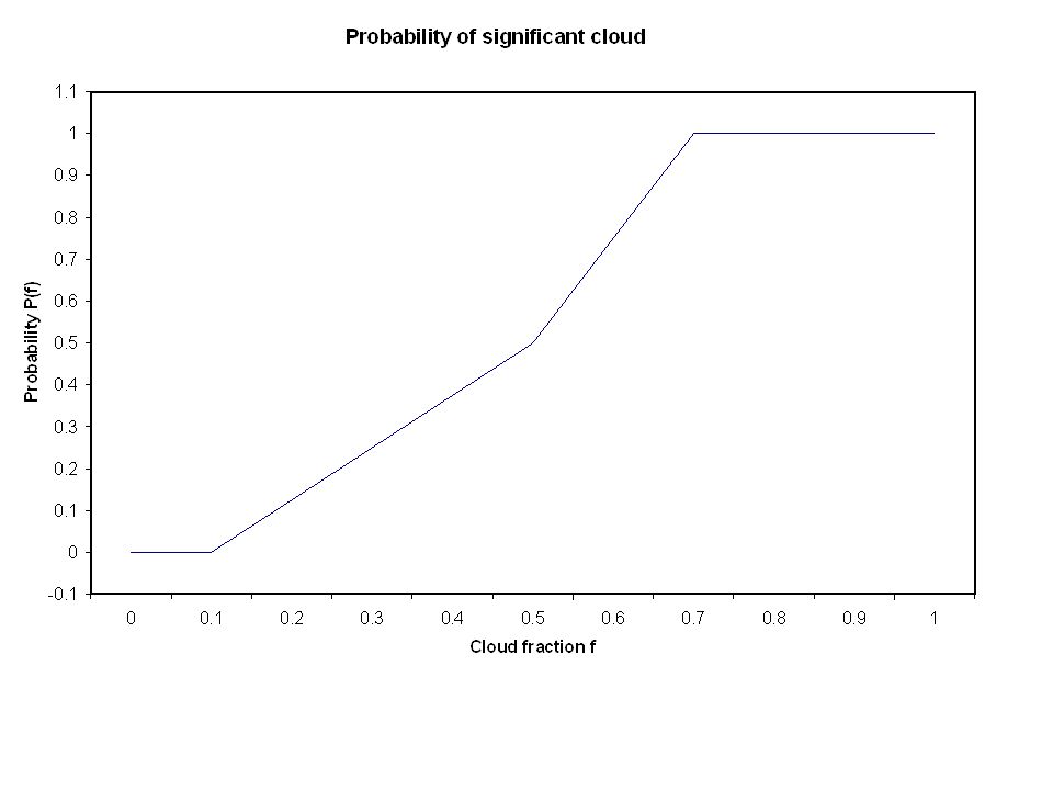
10. Simulation of Observations 1. All observations created using bilinear interpolation horizontally, log-linear interpolation vertically, linear interpolation in time 2. Radiance observations created using CRTM version 1.2 3. Clouds and precipitation are treated as elevated black bodies 4. No use of NR snow coverage 5. Locations for all “conventional” observations given by corresponding real ones, except no drift for RAOBS 6. SATWNDS not associated with trackable features in NR

12. Dependency of results on errors Consider Kalman filter applied to linear model Daley and Menard 1993 MWR

13. Simulation of Explicit Observation Errors 1.Some representativeness error implicitly present 2.Gaussian noise added to all observations 3.AIRS errors correlated between channels 4. Observational errors for SATWND and non-AIRS radiances horizontally correlated (using isotropic, Gaussian shapes) 5. Conventional soundings and SATWND observational errors vertically correlated (Gaussian shaped in log-p coordinate) 6. Tuning parameters are error standard deviations, fractions of variances for correlated components, vertical and horizontal length scales

14. AMSU-A NOAA-15RAOB GOES-IR Winds Standard deviations of Observation errors In GSI error tables (solid circles or lines) vs. For adding obs. errors (open circles or dashed lines)

15. Assimilation Metrics

16. Locations of QC-accepted observations for AIRS channel 295 at 18 UTC 12 July Real Simulated

17. Standard deviations of QC-accepted O-F values (Real vs. OSSE) AIR AQUA AMSU-A NOAA-15 RAOB U Wind RAOB q

19. Horizontal correlations of O-F AMSU-A NOAA-15 Chan 6 GLOB RAOB T 700 hPa NHET GOES-IR SATWND 300 hPa NHET GOES-IR SATWND 850 hPa NHET

20. Square roots of zonal means of temporal variances of analysis increments T OSSE T Real U OSSEU Real

21. Time mean Analysis increments T 850 hPa U 500 hPa OSSEReal

22. Forecast Metrics

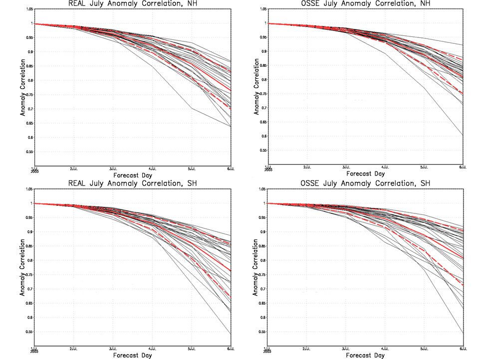
23. Real Control OSSE Control Mean anomaly correlations OSSE vs Real Data: Forecasts

25. Real Control OSSE Control January Forecasts

26. U-Wind RMS error: July Real Control OSSE Control Solid lines: 24 hour RMS error vs analysis Dashed lines: 120 hr forecast RMS error vs analysis

27. T RMS error: July Solid lines: 24 hour RMS error vs analysis Dashed lines: 120 hr forecast RMS error vs analysis Real Control OSSE Control

28. Real OSSE

29. Real OSSE

30. Real OSSE

31. Impact of obs errors on forecast

32. July Adjoint: dry error energy norm

34. Analysis and Forecast Error Vs. Nature Run

35. RMS OSSE Error vs NR, Temperature

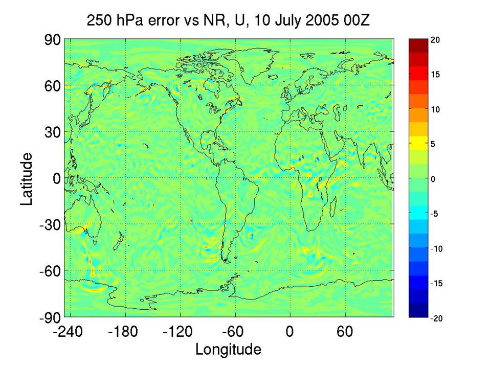
36. RMS Error vs NR, U wind

37. 400 hPa analysis error, U (m/s) July mean error vs NR

38. A-B at 400 hPa

39. Application: Characterization of analysis error (as an example of the kinds of calculations that can be performed)

40. Square roots of zonal means of temporal variances of U wind analysis error

41. Fractional reduction of zonal means of temporal variances of analysis errors compared with background errors uT

42. Horizontal spectra of analysis and analysis error (Spectra of time-mean fields subtracted) Rotational Wind 200 hPaDivergent Wind 200 hPa KE (J/kg) KE (J/kg) wave number n

43. Horizontal correlation length scales for v wind (Explicit bkg error vs. NMC method estimate) South PacificTropical Pacific

44. Application: Consideration of future instruments

45. ESA Aeolus Active measurements of wind from space – Measuring the Doppler shift imposed on lidar backscatter Launch delayed till late 2013 408 km, dawn-dusk, sun- synchronous orbit Wind measurements 90° off-track, 35° off-nadir – Nearly u @ equator No spaceborne heritage for DA development Utilize OSSE framework to generate realistic Aeolus proxy data – Lidar Performance Analysis Simulator (LIPAS), via KNMI (G.-J. Marseille & A. Stoffelen) Need proper sampling (spatial & vertical), yield, and errorcharacteristics

46. Assimilation Results Zonal Wind RMS Difference (ms -1 ) Large reductions of RMS seen over tropics Plots show reduction in analyzed u- wind RMS (compared to the NR as truth) by adding Aeolus observations to GMAO OSSE – Negative values indicate improvement Existing Observations primarily of mass field (passive satellite radiances) Winds cannot be inferred through balance assumptions

47. Assimilation Results Impact at 200 hPa consistent through troposphere Less impact towards surface – Less observations – Increased contamination Lesser impacts in N./S. hemispheres – Winds through mass-wind balance Less impact in mass fields, but still generally positive (not shown) Tropics (-30 º to 30 º ) NH Extratropics (30 º to 90 º ) SH Extratropics (-90 º to -30 º )

48. Conclusions, Caveats, and Future Efforts These results are overstated! – Error in simulated DWL observations inherently understated No added representativeness error – Error in Yield Lack of clouds in NR not accounted for in DWL obs simulation Shows expected result that largest impact is expected in tropics Future work – Include incorporation of L2B processing into DA System (GSI) Software release delayed due to change in instrument operations A necessary level of processing for use of data in near-realtime Will be included as part of outer loop processing – Redo experiment w/ simulator updated for change in instrument ops Simulator update in progress @ KNMI

49. Summary

50. 1. Fairly easy to match O-F covariances 2. Harder to match analysis increment statistics 3. Hardest to match forecast error metrics 4. Present OSSE framework validates reasonably well, but … 5. Some correctable deficiencies 6. Some puzzles

51. Continuing Development 1. New SATWND observation location determination based on NR 2.Fix surface wind observation simulator 3. Improve specification of land surface parameters for CRTM 4.Additional radiance observations 5.GPS observations 6.More complete tuning of conventional observation errors 7.Estimation of model error in OSSE framework 8.Use of other NR models 9.Demonstration of OSSE applications 10.Further examination of NMC method for estimating B

52. Extras

53. ‘Perfect’ Initial Conditions A grid of soundings with no error is ingested into the GSI – One sounding every other latitude and longitude from NR – Soundings extend to the top of the atmosphere – Ingested as type RAOB (120/220) – Intention is to drive the OSSE toward a ‘perfect’ initial condition Cycled from 15 Dec to 30 January Forecasts daily at 00Z

56. U-Wind RMS error vs NR OSSE Perfect OSSE Control Solid lines: analysis RMS error Dashed lines: 120 hr forecast RMS error

57. T RMS error vs NR Solid lines: analysis RMS error Dashed lines: 120 hr forecast RMS error OSSE Perfect OSSE Control

58. OSSE Perfect OSSE Control