Download presentation
Presentation is loading. Please wait.

1
ECE 802-604: Nanoelectronics Prof. Virginia Ayres Electrical & Computer Engineering Michigan State University ayresv@msu.edu

2
VM Ayres, ECE802-604, F13 Lecture 11, 03 Oct 13 In Chapter 02 in Datta: Transport: current I = GV V = IR => I = GV Velocity Energy levels M M(E) Conductance G = G C in a 1-DEG Example Pr. 2.1: 2-DEG-1-DEG-2-DEG Example: 3-DEG-1-DEG-3-DEG Transmission probability: the new ‘resistance’ How to evaluate the Transmission/Reflection probability T(N) for multiple scatterers T(L) in terms of a “how far do you get length” L 0 How to correctly measure I = GV Landauer-Buttiker: all things equal 3-, 4-point probe experiments: set-up and read out
 for multiple scatterers T(L) in terms of a how far do you get length L 0 How to correctly measure I = GV Landauer-Buttiker: all things equal 3-, 4-point probe experiments: set-up and read out.")
3
VM Ayres, ECE802-604, F13 Lec10: Scattering: Landauer formula for G

4
VM Ayres, ECE802-604, F13 Lec10: Scattering: Landauer formula for R … + ‘wire’ resistance: Dresselhaus

5
VM Ayres, ECE802-604, F13 E > barrier height V 0 E < barrier height V 0 Lec10: Modelled the scatterer X as a finite step potential in a certain region. Dresselhaus p. 144: static scattering, scattering by a potential in one dimension Modelled the wavelike e- as having energy E > or < V 0 and got a transmission probability T

6
VM Ayres, ECE802-604, F13 E > V 0 E < V 0 Point01: The phase and amplitude at electrode 2 can be obtained from the phase and amplitude at electrode 1 E > V 0 Phase and amplitude are the same E< V 0 Amplitude is reduced but phase is the same. 11 22 Phase: e- as wave is same at both contacts. This is the origin of the unchanged contact resistance G C - 1 = R C

7
VM Ayres, ECE802-604, F13 Point02: Everywhere: Transport is by occupying a discreet energy level, “channel”. Say that there are M channels in the 1-DEG. Dresselhaus Datta

8
VM Ayres, ECE802-604, F13 Point02: Everywhere: Transport is by occupying a discreet energy level, “channel”. Say that there are M channels in the 1-DEG. T is the transmission probability for a channel to go from electrode 1 to electrode 2, which is given by the sum of the sum of the transmission probability from the ith to the jth channel

9
VM Ayres, ECE802-604, F13 Point02: Everywhere: Transport is by occupying a discreet energy level, “channel”. Say that there are M channels in the 1-DEG. T is the transmission probability for a channel to go from electrode 1 to electrode 2, which is given by the sum of the sum of the transmission probability from the ith to the jth channel Clearly this e- didn’t make it. Reflections are the cause of resistance in the wire. … + ‘wire’ resistance: Dresselhaus

10
VM Ayres, ECE802-604, F13 Point02: Everywhere: Transport is by occupying a discreet energy level, “channel”. Say that there are M channels in the 1-DEG. T is the transmission probability for a channel to go from electrode 1 to electrode 2, which is given by the sum of the sum of the transmission probability from the ith to the jth channel Clearly this e- didn’t make it. Reflections are the cause of resistance in the wire. But don’t rule out scattering forward again. Versus

11
VM Ayres, ECE802-604, F13 Lecture 11, 03 Oct 13 In Chapter 02 in Datta: Transport: current I = GV V = IR => I = GV Velocity Energy levels M M(E) Conductance G = G C in a 1-DEG Example Pr. 2.1: 2-DEG-1-DEG-2-DEG Example: 3-DEG-1-DEG-3-DEG Transmission probability: the new ‘resistance’ How to evaluate the Transmission/Reflection probability T(N) for multiple scatterers T(L) in terms of a “how far do you get length” L 0 How to correctly measure I = GV Landauer-Buttiker: all things equal 3-, 4-point probe experiments: set-up and read out
 for multiple scatterers T(L) in terms of a how far do you get length L 0 How to correctly measure I = GV Landauer-Buttiker: all things equal 3-, 4-point probe experiments: set-up and read out.")
12
VM Ayres, ECE802-604, F13 This is a representation of 2 scatterers. Go from 2 scatterers to N scatterers per unit length L. What happens to the transmission probability T: R1R1 R2R2

13
VM Ayres, ECE802-604, F13 Transmission probability for 2 scatterers: T = T 12 : Include the forward reflections that rein forces the transmission: 1 back- forth then out 2 back- forth then out

14
VM Ayres, ECE802-604, F13 Transmission probability for 2 scatterers: T = T 12 : Eliminate R 1 and R 2 :

15
VM Ayres, ECE802-604, F13 Transmission probability for 2 scatterers: T = T 12 : Ratio the Reflection to the Transmission probability:

16
VM Ayres, ECE802-604, F13 Transmission probability for 2 scatterers: T = T 12 : That’s interesting. That Ratio is additive: Assuming that the scatterers are identical:

17
VM Ayres, ECE802-604, F13 Transmission probability for N identical scatterers: You’ll get the same result for N identical scatterers:

18
VM Ayres, ECE802-604, F13 Transmission probability for N identical scatterers: Now solve for transmission probability T(N):
:")
19
VM Ayres, ECE802-604, F13 Transmission probability T(N) => T(L): Re-write N in terms of = N/L: Define a “how far do you get length” L 0 : L 0 is similar to a mean free path L m but in terms of T versus lots/few R
 => T(L): Re-write N in terms of = N/L: Define a how far do you get length L 0 : L 0 is similar to a mean free path L m but in terms of T versus lots/few R")
20
VM Ayres, ECE802-604, F13 Transmission probability T(N) => T(L): Therefore: with:
 => T(L): Therefore: with:")
21
VM Ayres, ECE802-604, F13 Transmission probability T(N) => T(L):
 => T(L):")
22
VM Ayres, ECE802-604, F13 Lecture 11, 03 Oct 13 In Chapter 02 in Datta: Transport: current I = GV V = IR => I = GV Velocity Energy levels M M(E) Conductance G = G C in a 1-DEG Example Pr. 2.1: 2-DEG-1-DEG-2-DEG Example: 3-DEG-1-DEG-3-DEG Transmission probability: the new ‘resistance’ How to evaluate the Transmission/Reflection probability T(N) for multiple scatterers T(L) in terms of a “how far do you get length” L 0 How to correctly measure I = GV Landauer-Buttiker: all things equal 3-, 4-point probe experiments: set-up and read out
 for multiple scatterers T(L) in terms of a how far do you get length L 0 How to correctly measure I = GV Landauer-Buttiker: all things equal 3-, 4-point probe experiments: set-up and read out.")
23
VM Ayres, ECE802-604, F13 Now relate the transmission probability T(N) or T(L) to an e- current I using Landauer’s formula for G:
 or T(L) to an e- current I using Landauer’s formula for G:")
24
VM Ayres, ECE802-604, F13 Add probes: 3-point configurations:

25
VM Ayres, ECE802-604, F13 Add probes: 4-point configurations:

26
VM Ayres, ECE802-604, F13 h Landauer-Buttiker formalism: Very briefly: why:

27
VM Ayres, ECE802-604, F13 Landauer-Buttiker formalism: Very briefly: why: 2/ Due to a physical bending, probe P1 couples preferentially to -k x states, while probe P2 couples preferentially to +k x states. You could read normal, very low or negative resistance depending on T. 3/ How close is your probe to a scatterer: e- wave interference zero reading?

28
VM Ayres, ECE802-604, F13 Landauer-Buttiker formalism: Very briefly: why:

29
VM Ayres, ECE802-604, F13 Landauer-Buttiker formalism: how: q <- p is from p to q, where p and q are any of the terminals.

30
VM Ayres, ECE802-604, F13 Landauer-Buttiker formalism: how:

31
VM Ayres, ECE802-604, F13 Landauer-Buttiker formalism: how:

32
VM Ayres, ECE802-604, F13 Landauer-Buttiker formalism: how:

33
VM Ayres, ECE802-604, F13 Landauer-Buttiker formalism: how: GOAL: Find resistance R

34
VM Ayres, ECE802-604, F13 Example: 3 point probe-a Find R for this circuit!

35
VM Ayres, ECE802-604, F13 qqq

36
qqq

37
qqq

38
Landauer-Buttiker set-up is complete

39
VM Ayres, ECE802-604, F13

47
In V 1 eq’n ?

48
VM Ayres, ECE802-604, F13

54
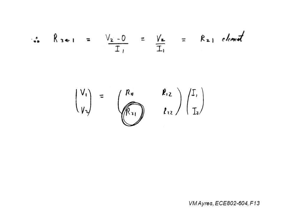
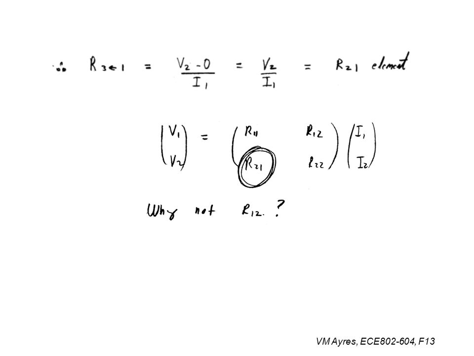
= R 21 R 3terminal = R 3t

55
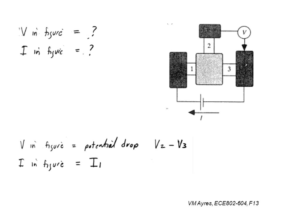
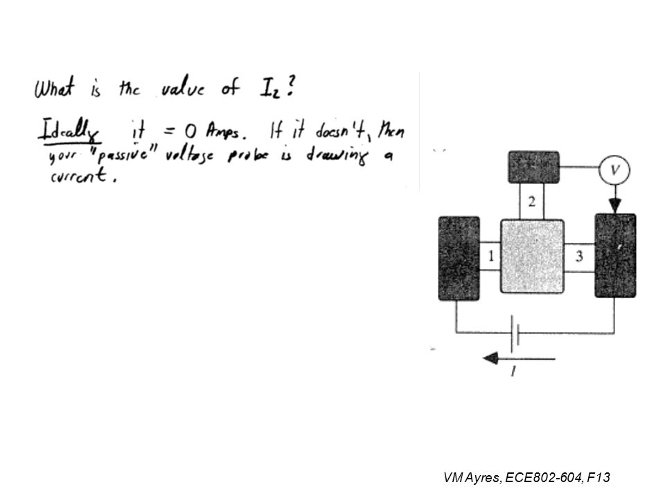
VM Ayres, ECE802-604, F13 Example: 3 point probe-b Question: How would you find R for this configuration? Answer: a/ Choose: V 3 = 0 b/ Choose: ideal I 1 = 0 c/ From I-V 2x2 matrix equations, identify the R that you want as:

56
VM Ayres, ECE802-604, F13 Example: 3 point probe-b Question: How would you find R for this configuration? Answer: a/ Choose: V 3 = 0 b/ Choose: ideal I 1 = 0 c/ From I-V 2x2 matrix equations, identify the R that you want as: From: V’ = V 1 – V 3 =R 11 I 1 + R 12 I 2

Similar presentations


![“Over the weekend, I reviewed the exam and figured out what concepts I don’t understand.” A] true B] false 1 point for either answer.](/24/7048369/big_thumb.jpg "“Over the weekend, I reviewed the exam and figured out what concepts I don’t understand.” A] true B] false 1 point for either answer.>")


