1. Model Building For ARIMA time series
Consists of three steps
Identification
Estimation
Diagnostic checking

2. Determination of p, d and q
ARIMA Model building
Identification
Determination of p, d and q

3. To identify an ARIMA(p,d,q) we use extensively
the autocorrelation function
{rh : - < h < }
and
the partial autocorrelation function,
{Fkk: 0  k < }.

4. The definition of the sample covariance function
{Cx(h) : - < h < }
and the sample autocorrelation function
{rh: - < h < }
are given below:
The divisor is T, some statisticians use T – h (If T is large, both give approximately the same results.)

5. It can be shown that:
Thus
Assuming rk = 0 for k > q

6. The sample partial autocorrelation function is defined by:

7. It can be shown that:

8. Identification of an Arima process
Determining the values of p,d,q

9. Recall that if a process is stationary one of the roots of the autoregressive operator is equal to one.
This will cause the limiting value of the autocorrelation function to be non-zero.
Thus a nonstationary process is identified by an autocorrelation function that does not tail away to zero quickly or cut-off after a finite number of steps.

10. To determine the value of d
Note: the autocorrelation function for a stationary ARMA time series satisfies the following difference equation
The solution to this equation has general form
where r1, r2, r1, … rp, are the roots of the polynomial

11. For a stationary ARMA time series
The roots r1, r2, r1, … rp, have absolute value greater than 1.
Therefore
If the ARMA time series is non-stationary
some of the roots r1, r2, r1, … rp, have absolute value equal to 1, and

12. stationary
non-stationary

13. If the process is non-stationary then first differences of the series are computed to determine if that operation results in a stationary series.
The process is continued until a stationary time series is found.
This then determines the value of d.

14. Determination of the values of p and q.
Identification
Determination of the values of p and q.

15. To determine the value of p and q we use the graphical properties of the autocorrelation function and the partial autocorrelation function.
Again recall the following:

16. Patterns of the ACF and PACF of AR(2) Time Series
More specically some typical patterns of the autocorrelation function and the partial autocorrelation function for some important ARMA series are as follows:
Patterns of the ACF and PACF of AR(2) Time Series
In the shaded region the roots of the AR operator are complex

17. Patterns of the ACF and PACF of MA(2) Time Series
In the shaded region the roots of the MA operator are complex

18. Patterns of the ACF and PACF of ARMA(1.1) Time Series
Note: The patterns exhibited by the ACF and the PACF give important and useful information relating to the values of the parameters of the time series.

19. Summary: To determine p and q.
Use the following table.
MA(q)
AR(p)
ARMA(p,q)
ACF
Cuts after q
Tails off
PACF
Cuts after p
Note: Usually p + q ≤ 4. There is no harm in over identifying the time series. (allowing more parameters in the model than necessary. We can always test to determine if the extra parameters are zero.)

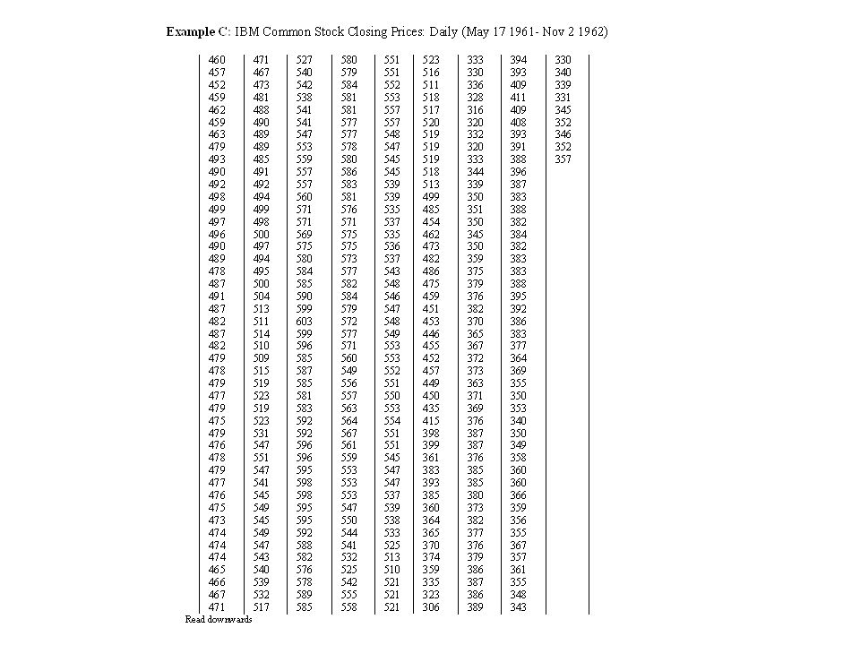
20. Examples

22. The data

24. The data

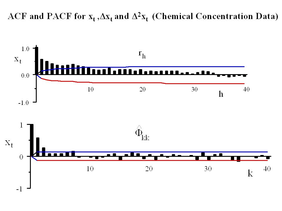
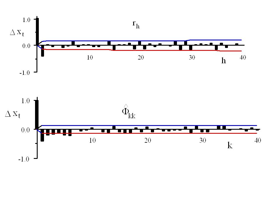
31. Possible Identifications
d = 0, p = 1, q= 1
d = 1, p = 0, q= 1

33. ACF and PACF for xt ,Dxt and D2xt (Sunspot Data)

36. Possible Identification
d = 0, p = 2, q= 0

38. ACF and PACF for xt ,Dxt and D2xt (IBM Stock Price Data)

41. Possible Identification
d = 1, p =0, q= 0

42. Estimation
of ARIMA parameters

43. Preliminary Estimation
Using the Method of moments
Equate sample statistics to population paramaters

44. Estimation of parameters of an MA(q) series
The theoretical autocorrelation function in terms the parameters of an MA(q) process is given by.
To estimate a1, a2, … , aq we solve the system of equations:

45. This set of equations is non-linear and generally very difficult to solve
For q = 1 the equation becomes:
Thus or
This equation has the two solutions
One solution will result in the MA(1) time series being invertible

46. For q = 2 the equations become:

47. Estimation of parameters of an ARMA(p,q) series
We use a similar technique.
Namely: Obtain an expression for rh in terms b1, b2 , ... , bp ; a1, a1, ... , aq of and set up q + p equations for the estimates of b1, b2 , ... , bp ; a1, a2, ... , aq by replacing rh by rh.

48. Estimation of parameters of an ARMA(p,q) series
Example: The ARMA(1,1) process
The expression for r1 and r2 in terms of b1 and a1 are:
Further

49. Thus the expression for the estimates of b1, a1, and s2 are :

50. Hence or
This is a quadratic equation which can be solved

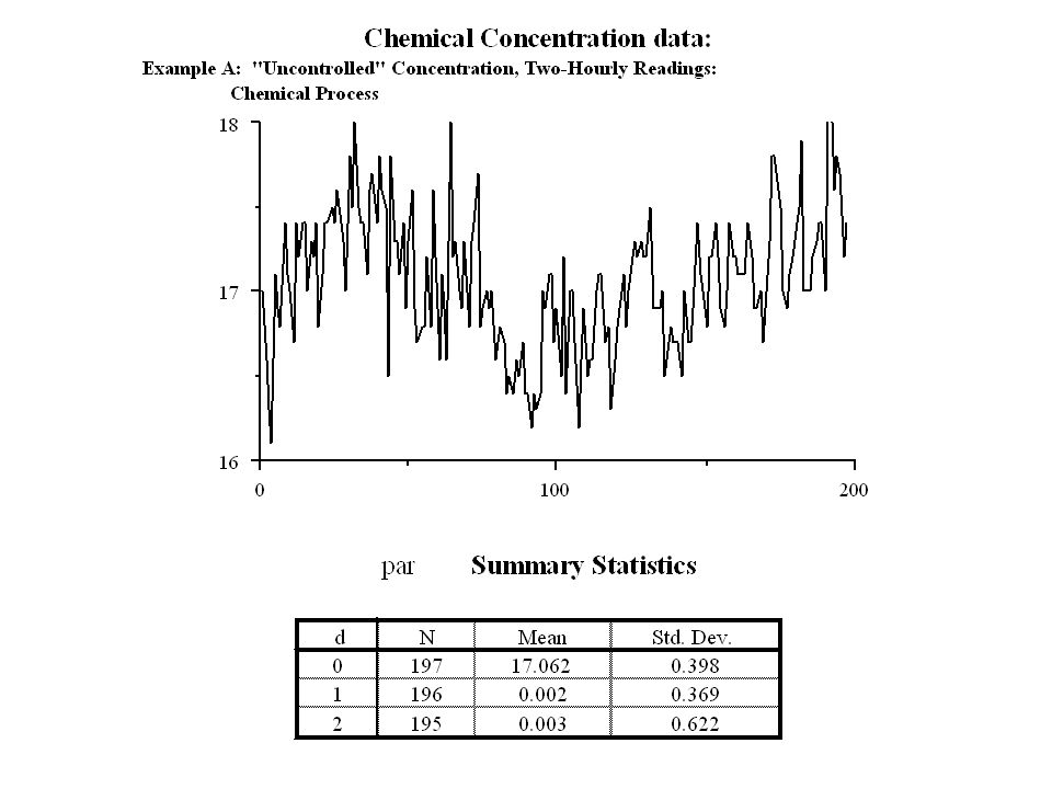
51. Example (ChemicalConcentration Data)
the time series was identified as either an ARIMA(1,0,1) time series or an ARIMA(0,1,1) series.
If we use the first identification then series xt is an ARMA(1,1) series.

52. Identifying the series xt is an ARMA(1,1) series.
The autocorrelation at lag 1 is r1 = and the autocorrelation at lag 2 is r2 =
Thus the estimate of b1 is 0.495/0.570 = 0.87.
Also the quadratic equation
becomes
which has the two solutions and Again we select as our estimate of a1 to be the solution -0.48, resulting in an invertible estimated series.

53. Since d = m(1 - b1) the estimate of d can be computed as follows:
Thus the identified model in this case is
xt = 0.87 xt-1 + ut ut

54. If we use the second identification then series
Dxt = xt – xt-1 is an MA(1) series.
Thus the estimate of a1 is:
The value of r1 =
Thus the estimate of a1 is:
The estimate of a1 = -0.53, corresponds to an invertible time series. This is the solution that we will choose

55. The estimate of the parameter m is the sample mean.
Thus the identified model in this case is:
Dxt = ut ut or
xt = xt-1 + ut ut
This compares with the other identification:
(An ARIMA(0,1,1) model)
xt = 0.87 xt-1 + ut ut
(An ARIMA(1,0,1) model)

56. Preliminary Estimation
of the Parameters of an AR(p) Process

57. The regression coefficients b1, b2, …
The regression coefficients b1, b2, …., bp and the auto correlation function rh satisfy the Yule-Walker equations:
and

58. The Yule-Walker equations can be used to estimate the regression coefficients b1, b2, …., bp using the sample auto correlation function rh by replacing rh with rh.
and

59. Example
Considering the data in example 1 (Sunspot Data) the time series was identified as an AR(2) time series .
The autocorrelation at lag 1 is r1 = and the autocorrelation at lag 2 is r2 =
The equations for the estimators of the parameters of this series are
which has solution
Since d = m( 1 -b1 - b2) then it can be estimated as follows:

60. Thus the identified model in this case is
xt = xt xt-2 + ut +14.9

61. Maximum Likelihood Estimation
of the parameters of an ARMA(p,q) Series

62. The method of Maximum Likelihood Estimation selects as estimators of a set of parameters q1,q2, ... , qk , the values that maximize
L(q1,q2, ... , qk) = f(x1,x2, ... , xN;q1,q2, ... , qk)
where f(x1,x2, ... , xN;q1,q2, ... , qk) is the joint density function of the observations x1,x2, ... , xN.
L(q1,q2, ... , qk) is called the Likelihood function.

63. It is important to note that:
finding the values -q1,q2, ... , qk- to maximize L(q1,q2, ... , qk) is equivalent to finding the values to maximize l(q1,q2, ... , qk) = ln L(q1,q2, ... , qk).
l(q1,q2, ... , qk) is called the log-Likelihood function.

64. Again let {ut : t ÎT} be identically distributed and uncorrelated with mean zero. In addition assume that each is normally distributed .
Consider the time series {xt : t ÎT} defined by the equation:
(*) xt = b1xt-1 + b2xt bpxt-p + d + ut
+a1ut-1 + a2ut aqut-q

65. Assume that x1, x2, ...,xN are observations on the time series up to time t = N.
To estimate the p + q + 2 parameters b1, b2, ... ,bp ; a1, a2, ... ,aq ; d , s2 by the method of Maximum Likelihood estimation we need to find the joint density function of x1, x2, ...,xN
f(x1, x2, ..., xN |b1, b2, ... ,bp ; a1, a2, ... ,aq , d, s2)
= f(x| b, a, d ,s2).

66. We know that u1, u2, ...,uN are independent normal with mean zero and variance s2.
Thus the joint density function of u1, u2, ...,uN is g(u1, u2, ...,uN ; s2) = g(u ; s2) is given by.

67. It is difficult to determine the exact density function of x1,x2,
It is difficult to determine the exact density function of x1,x2, ... , xN from this information however if we assume that p starting values on the x-process x* = (x1-p,x2-p, ... , xo) and q starting values on the u-process u* = (u1-q,u2-q, ... , uo) have been observed then the conditional distribution of x = (x1,x2, ... , xN) given x* = (x1-p,x2-p, ... , xo) and u* = (u1-q,u2-q, ... , uo) can easily be determined.

68. The system of equations :
x1 = b1x0 + b2x bpx1-p + d + u1 +a1u0
+ a2u aqu1-q
x2 = b1x1 + b2x bpx2-p + d + u2 +a1u1
+ a2u aqu2-q
...
xN= b1xN-1 + b2xN bpxN-p + d + uN
+a1uN-1 + a2uN aquN-q

69. can be solved for:
u1 = u1 (x, x*, u*; b, a, d)
u2 = u2 (x, x*, u*; b, a, d)
...
uN = uN (x, x*, u*; b, a, d)
(The jacobian of the transformation is 1)

70. Then the joint density of x given x* and u* is given by:

71. Let:
= “conditional likelihood function”

72. “conditional log likelihood function” =

73. The values that maximize
are the values
that minimize
with

74. Comment:
The minimization of:
Requires a iterative numerical minimization procedure to find:
Steepest descent
Simulated annealing
etc

75. Comment:
The computation of:
for specific values of
can be achieved by using the forecast equations

76. Comment:
The minimization of :
assumes we know the value of starting values of the time series {xt| t  T} and {ut| t  T}
Namely x* and u*.

77. Approaches:
Use estimated values:
Use forecasting and backcasting equations to estimate the values:

78. Backcasting: If the time series {xt|t  T} satisfies the equation:
It can also be shown to satisfy the equation:
Both equations result in a time series with the same mean, variance and autocorrelation function:
In the same way that the first equation can be used to forecast into the future the second equation can be used to backcast into the past:

79. Approaches to handling starting values of the series {xt|t  T} and {ut|t  T}
Initially start with the values:
Estimate the parameters of the model using Maximum Likelihood estimation and the conditional Likelihood function.
Use the estimated parameters to backcast the components of x*. The backcasted components of u* will still be zero.

80. Repeat steps 2 and 3 until the estimates stablize.
This algorithm is an application of the E-M algorithm
This general algorithm is frequently used when there are missing values.
The E stands for Expectation (using a model to estimate the missing values)
The M stands for Maximum Likelihood Estimation, the process used to estimate the parameters of the model.

81. Some Examples using:
Minitab
Statistica
S-Plus
SAS