1. Quantity of Water and Wastewater CE 547

2. Probability Quantity of Water Types of Wastewater Sources of Wastewater Population Projection Deriving Design Flows of Wastewater Contents

3. Probability 1. Values Equaled or Exceeded  One element equal to the value  Elements exceeding the value Prob (value equaled or exceeded) = Prob (value equaled) + Prob (value exceeded) – Prob (value equaled  value exceeded)

4. Since the intersection probability = zero Then, Prob (value exceeded) = Prob (value 1 exceeded) + Prob (value 2 exceeded) +…+ Prob (value  exceeded) Prob (value equaled or exceeded) = Prob (value equaled) + Prob (value 1 exceeded) + Prob (value 2 exceeded) +…+ Prob (value  exceeded)

5. Probability 2. Derivation of Probability from Recorded Observation (E) = occurrence of the event  = no of units favorable  s = total possible number of events

6. Determination of  s  Costly  Not available So,  approx is used instead. If  approx is small, then the probability produced might be wrong. To correct this, 1 is added to the denominator

7. Example 1

10. Probability 3. Values Equaled or Not Exceeded Values equaled or not exceeded is just the reverse of values equaled or exceeded Prob (value equaled or not exceeded) = Prob (value equaled ) + Prob (value 1 not exceeded) + Prob (value 2 not exceeded) +….+ Prob (value  not exceeded)

11. Example 2

13. Quantity of Water

14. Quantities of water and wastewater are required by designers. Examples: I. Maximum daily flow is used to design  community water supplies  water intakes  wells  treatment plants  pumping stations  transmission lines Hourly variations are handled by storage.

15. II. Water distribution systems are designed on the basis of the MAXIMUM DAY PLUS FLOW FOR FIRE FIGHTING or on the basis of the MAXIMUM HOURLY whichever is greater Another parameter needed by designers is the DESIGN PERIOD

16. What is Design Period? Time from the initial design years to the time that the facility is to receive the final design flows. Facilities would be designed at stages. It starts smaller and it gets bigger with time (staging period) due to increase in population.

17. Staging Periods (Table page 87)

18. Design Periods (Table page 87)

19. Average Rates of Water Use (Tables page 88 and 89)

22. Types and Sources of Wastewater

23. Types of Wastewater (two main types)  Sanitary (from human activities)  Residential (domestic wastewater)  Industries (industrial sanitary wastewater)  Industrial (from manufacturing processes) Infiltration: water entering the sewer through cracks or imperfect connections Inflow: water entering the sewer through openings that were not meant for that purpose

24. Sources of Wastewater (Tables page 91 to 93) Residential Residential Commercial Commercial Institutional Institutional Recreational Recreational Industrial Industrial

25. Population Prediction

26. Why is it Needed? To determine the design flows for a community Several methods are used  Arithmetic method  Geometric method  Declining rate of increase method  Logistic method  Graphical comparison method

27. Arithmetic Method The population at present increase at a constant rate The method is applicable for short-term projections (  30 years)

29. Example

30. The population for City A is as follows: 198015,000 199018,000 What will be the population in 2000?

31. Solution

32. Geometric Method  The population at present increase in proportion to the number at present  Used for short-term projections

34. Example

35. Repeat the previous example using the geometric method.

36. Solution

37. Declining-Rate-of-Increase Method  The population will reach a saturation value  The rate of increase will decline until it becomes zero at saturation

39. Example

40. If the population of City A is as follows: 198015,000 199018,000 200020,000 What will be the population in 2020?

41. Solution

42. Logistic Method If environmental conditions are optimum, population will increase at geometric rate. In reality, this will be slowed down due to environmental constraints such as:  Decreasing rate of food supplies  Over-crowding  Death

43. According to the geometric method: To enforce the environmental constraints, k g P should be multiplied by a factor less than 1. In logistic method, the factor 1 is reduced by P/K. Where K = carrying capacity of the environment (1-P/K) = environmental resistance

44. Therefore, the logistic equation becomes: Note that k g changed to k l. Re-arrange:

45. Substitute in (1) and integrate twice:

46. Solve for k l

47. Example

48. If the population of City A is as follows: 198015,000 199018,000 200020,000 What will be the population in 2020?

50. Graphical Comparison Method Plot the population of the given City along with other cities which are larger in size but have similar characteristics. This method extends a line reflecting the slope of each ten (10) year interval between censuses. An average line is then determined to reflect the population estimate of future years. Plot the population of the given City along with other cities which are larger in size but have similar characteristics. This method extends a line reflecting the slope of each ten (10) year interval between censuses. An average line is then determined to reflect the population estimate of future years. This method involves extension of the population-time curve of the city C (under consideration) based on comparison with population-time curves of similar but larger cities A and B. These larger cities A and B must have reached the present population of the city C one or more decades ago. Starting from the point on curve C representing the present population, the curves corresponding to the growths of A and B after their reaching that population are plotted. The extension of the curve C is modified keeping in view the projections offered by A and B as well as other related conditions.

51. Deriving Design Flows of Wastewater Types of flow rates used in the design:  Average daily flow rate  Maximum daily flow rate  Peak hourly flow rate  Minimum daily flow rate  Minimum hourly flow rate  Sustained high flow rate  Sustained low flow rate

52. What is needed to determine these flow rates?  Statistically sufficient amount of data should be available Where to get data from? 1.Literature (least desirable) 2.Treatment plant records 3.Field surveys (costly and short-term) 1 and 2 are not recommended because  Habits of people are different  Characteristics of land area are different (precipitation which affects infiltration into the sewer)

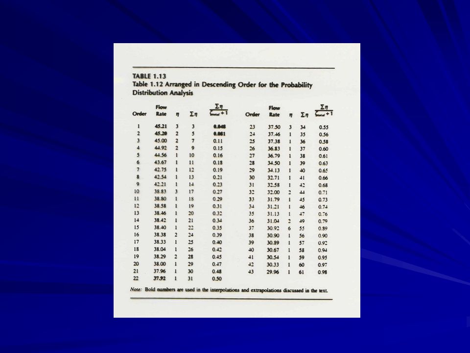
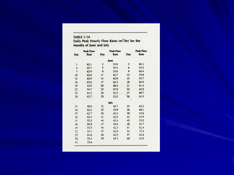
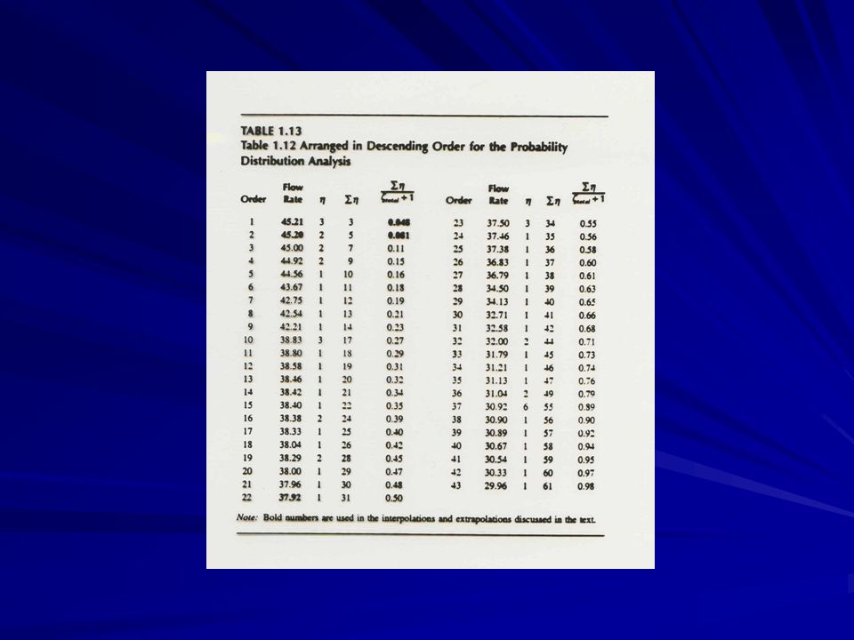
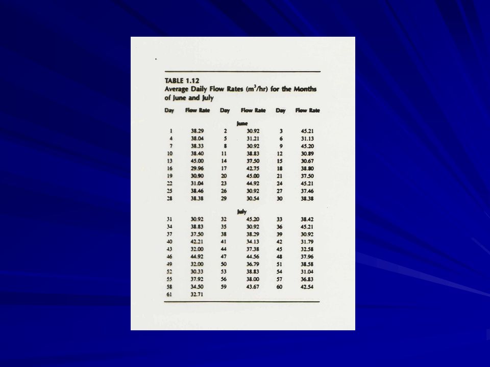
53. Average Daily Flow Rate Average flow rate corresponds to 50% probability If we have the data shown in Figures 1.6 and 1.7 for June and July, then the daily average can be calculated using the graphical method shown in Figure 1.8. This method should be used for each individual day. Tabulate the results (Table 1.12):  Arrange the data in ascending or descending order  Calculate probability distribution  Average flow is at 50% probability  If 50% is not available, then interpolate (Table 1.13)

58. Peak Hourly Flow Rate  Corresponds to probability of zero  Find peak hourly flow rate for each day from original data  Tabulate the results (Table 1.14)  Arrange in descending order  Read or extrapolate flow rate with probability of zero (Table 1.15)

61. Maximum Daily Flow Rate  Same data used for average daily flow rate (Table 1.13)  Corresponds to zero probability  Read or extrapolate flow rate at probability of zero

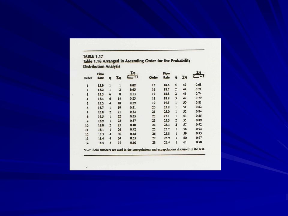
63. Minimum Hourly Flow Rate  Obtain the lowest flow each day from original data (Figures 1.6 and 1.7)  Tabulate the daily minimum hourly flow rates (Table 1.16)  Arrange in ascending order  Read or extrapolate flow rate at probability of zero

66. Minimum Daily Flow Rate  Use data on average flow rates (Table 1.12)  Rearrange in ascending order (Table 1.18)  Read or extrapolate flow rate at probability of zero

69. Sustained Peak Flow rate and Sustained Minimum Flow Rate Define a parameter called “moving average” Element No123456 Element Value232143323426 1 st moving average = (23+21+43)/3 = 29232143 2 nd moving average = (21+43+32)/3 = 32214332 3 rd moving average = (43+32+34)/3 = 36.3433234 4 th moving average = (32+34+26)/3 = 30.7323426

70. No of moving averages If  e = no of elements (6)  me = no of moving elements to be averaged  mav =  e -  me +1 where  mav = no of moving averages

71. How to find Sustained Peak Flow Rate?  Tabulate data (Table 1.12)  Find moving average (Table 1.20)  Arrange moving averages in descending order (Table 1.21)  Read or extrapolate flow rate at probability of zero

75. So, if: X0 38.240.02 38.120.04 Then,

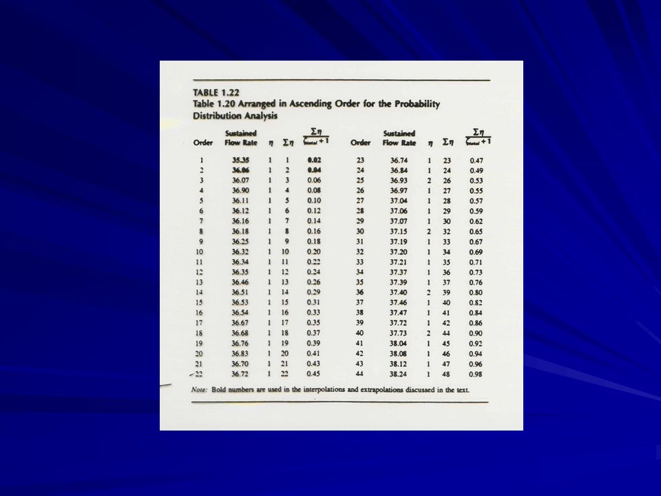
76. How to find Sustained Minimum Flow Rate?  Tabulate data (Table 1.12)  Find moving average (Table 1.20)  Arrange moving averages in ascending order (Table 1.22)  Read or extrapolate flow rate at probability of zero

80. So, if: X0 35.350.02 30.060.04 Then,