Download presentation
Presentation is loading. Please wait.

1
Summary The long-run model determines potential output and the long-run rate of inflation. The short-run model determines current output and current inflation. In any given year, output consists of two components: The long-run potential output Short-run output

2
Short run output Recession:
Is the percentage difference between actual and potential output. Is positive when the economy is booming. Is negative when the economy is slumping. Recession: Our Definition: A period when actual output falls below potential Short-run output becomes negative (Ỹ < 0) Usual Definition (Roughly) 2 Quarters of negative GDP. Declared by the NBER Business Cycle Dating Committee. (ΔY < 0)
 Usual Definition. (Roughly) 2 Quarters of negative GDP. Declared by the NBER Business Cycle Dating Committee. (ΔY < 0)")
3
Short-run fluctuation
The difference in actual and potential output, expressed as a percentage of potential output Referred to as “detrended output” or short-run output: The right-hand side of the bottom equation is the percentage change (A – B)/B.
/B.")
4
Figure 9.1 shows a stylized graph of actual and potential output (panel a), as well as a measure of the implied short-run fluctuations (panel b). A key thing to notice in this figure is that Y(tilde) looks much like actual output. When we remove the long-run trend associated with economic growth (potential output), what remains are the ups and downs of economic fluctuations (panel b). For this reason, economists often refer to Y(tilde) as “detrended output,” or short-run output. When an economy is booming, actual output is above potential, and Y(tilde) is positive. When an economy is in recession, actual output is less than potential output, and Y(tilde) is negative.
 looks much like actual output. When we remove the long-run trend associated with economic growth (potential output), what remains are the ups and downs of economic fluctuations (panel b). For this reason, economists often refer to Y(tilde) as detrended output, or short-run output. When an economy is booming, actual output is above potential, and Y(tilde) is positive. When an economy is in recession, actual output is less than potential output, and Y(tilde) is negative..")
5
Ȳ ΔY<0 ΔY>0 ΔY<0 but Ỹ > 0 ΔY>0 but Ỹ < 0 Ỹ < 0
Recession Ends ΔY>0 but Ỹ < 0

9
A recession: During a recession:
Begins when actual output falls below potential, and short-run output becomes negative. Ends when short-run output starts to rise and become less negative. During a recession: Output is usually below potential for approximately two years, which results in a loss of about $2,400 per person. Between 1.5 million and 3 million jobs are lost. Note, however, that the costs of short-term fluctuations are much less than these indicators suggest because they do not incorporate the benefits of a boom.

10
Measuring Potential Output
There is no directly observable measure of potential output in an economy. Ways to measure potential output: Assume a perfectly smooth trend passes through quarterly movements of real GDP. Take averages of the surrounding actual GDP numbers. Absent any way to measure potential output, economists must consult a variety of indicators. Current GDP numbers can be obtained quite easily from statistical agencies in virtually any economy: they are simply careful measures of what is actually produced. But how do we measure potential output, an economic construct that is not directly observable? One way is to assume there’s a perfectly smooth trend passing through the quarter-to-quarter movements in real GDP. An alternative is to take averages of the surrounding actual GDP numbers.

11
Because of the magnitude of economic growth, actual and potential output look quite similar on this time scale.

12
Figure 9.3 shades periods during which the economy was in a recession.
In general, a recession begins when actual output falls below potential; that is, when short-run output becomes negative. The recession is usually declared to be over when short-run output starts to rise and become less negative, before output returns to potential. Since 1950, the fluctuations in real GDP have usually ranged from about -4 percent to +4 percent. The deepest recession before the recent financial crisis occurred in 1980–82, when output fell to 5 percent below potential. The recessions in 1990–91 and 2001 were substantially milder. In contrast, the most recent recession, which began in December 2007, shows a level of output by the end of 2009 that was more than 6 percent below potential. In a typical recession, output falls below potential for about two years, first during the recession itself and then as the economy recovers back to potential. If we add up the lost output over the entire length of a typical recession, about 6 percent of GDP is forgone. To put this number into perspective, recall that U.S. GDP in 2009 was about $14 trillion, and 6 percent of this is about $840 billion. Since the U.S. population is about 300 million, the loss works out to about $2,800 per person, or about $11,000 per family of four. On average, then, a recession is quite costly. In addition, the decline in income is typically not spread evenly across the population. To the extent that it’s concentrated in particular regions, industries, and families, the costs to those affected can be even larger.

13
9.3 The Short-Run Model Short-run model features:
Open economy exists where global booms and recessions impact the local economy. The economy will exhibit long-run growth and fluctuations. Central Bank manages monetary policy to smooth fluctuations.

14
The short-run model is based on three premises:
1. The economy is constantly being hit by shocks: Shocks: factors that cause fluctuations in output or inflation. 2. Monetary and fiscal policies affect output: Policymakers may be able to neutralize shocks to the economy. 1. The economy is constantly being hit by shocks. These economic shocks include changes in oil prices, disruptions in financial markets, the development of new technologies, changes in military spending, and natural disasters. Such shocks can push actual output away from potential output and/or move the inflation rate away from its long-run value. 2. Monetary and fiscal policy affect output. The government has monetary and fiscal tools at its disposal that can affect the amount of economic activity in the short run. In principle, this means policymakers might be able to neutralize shocks to the economy. For example, if the economy is hit with a negative shock like a rise in oil prices, the government may use monetary policy to stimulate the economy and keep output from falling below potential.

15
3. There is a dynamic trade-off between output and inflation:
The Phillips curve is the dynamic trade-off between output and inflation. The government does not want to keep actual GDP as high as possible because a booming economy leads to an increase in the inflation rate If inflation is high, a recession is usually required to lower it. 3. There is a dynamic trade-off between output and inflation. If the government can affect output, wouldn’t it try to keep actual GDP as high as possible? This is an important question and goes to the heart of our short-run model. The answer is no, and the reason lies in this trade-off. A booming economy today — in which the economy is producing more than its potential output — leads to an increase in the inflation rate. Conversely, if the inflation rate is high and policymakers want to lower it, a recession is typically required. This trade-off is known as the Phillips curve, named after the New Zealand–born economist A. W. Phillips, who first identified this kind of trade-off in 1958.

16
Philips curve

17
The Empirical Fit of the Phillips Curve
Empirically, the slope is approximately one-half. Meaning: if output exceeds potential by 2 percent, the inflation rate increases one percentage point. Empirically means that we are fitting a curve to recorded data.

18
Teaching Tip: Have the students locate the dots for 1979, 1980, 1981, and 1982 to show the effect of the 1979 Monetary Policy. Figure 9.7 shows the empirical version of the Phillips curve for the U.S. economy since 1960; that is, it plots historical data on the change in inflation and short-run output for each year. As shown in the graph, in years when output is above potential, the inflation rate has typically risen. Conversely, when the economy is slumping, the inflation rate has typically declined. On average, the slope of this relationship is about 1/2, so that when output exceeds potential by 2 percent, the inflation rate rises by about 1 percentage point. The data point for 2009, in the lower left part of the figure, provides a nice illustration. Actual output was far below potential, and the inflation rate declined sharply. Compare to Figure 9.5 to see this more directly.) The graph also shows that in many years, the change in the inflation rate has been higher or lower than what the Phillips curve predicts. In part, this is because of shocks. For example, in both 1974 and 1979, oil prices rose sharply on world markets, leading the U.S. inflation rate to rise by more than would be implied by its level of output.
 The graph also shows that in many years, the change in the inflation rate has been higher or lower than what the Phillips curve predicts. In part, this is because of shocks. For example, in both 1974 and 1979, oil prices rose sharply on world markets, leading the U.S. inflation rate to rise by more than would be implied by its level of output.")
19
How the Short-Run Model Works
Assume policymakers can select short-run output through monetary policy Example: 1979: inflation was increasing because of oil prices Monetary Policy: raise interest rates What happens? Recession! The unintended consequence is that the policy induces a recession because higher interest rates discourage investment. As output declines, firms face lower demand and reduce costs so inflation falls dramatically.

21
The Phillips curve relates the change in the inflation rate to the amount of economic activity. In a booming economy (Y > 0), inflation rises. In a slumping economy (Y < 0), inflation falls.
, inflation rises. In a slumping economy (Y < 0), inflation falls..")
22
Important thing about the Philip Curve
This is about accelerating and decelerating inflation. This is a change in the change of the price level Is the Philips Curve fixed? Supply Shocks. Expectations.

23
Okun’s law

24
Okun’s law says that for each percentage point that output is below potential, the unemployment rate exceeds its long-run level by half a percentage point. The long-run (natural) unemployment rate u is measured as the average rate in the surrounding period. What we see in Figure 9.8 is a tight, negative relationship between output and unemployment. If output is above potential, the economy is booming and the unemployment rate is low. If output is below potential, the economy is in a recession and unemployment is high.

25
Cyclical unemployment
Okun’s Law Cyclical unemployment Current rate of unemployment Short-run output Natural rate of unemployment Teaching Tip: Click through to label terms. Okun’s law provides a way to relate output and unemployment. Plotting data (empirical again!) for cyclical unemployment and short-run output yields Okun’s law, which says that the difference between the unemployment rate and the natural rate of unemployment is equal to negative one-half times short-run output.
 for cyclical unemployment and short-run output yields Okun’s law, which says that the difference between the unemployment rate and the natural rate of unemployment is equal to negative one-half times short-run output.")
26
Okun’s Law 1960 Recession

27
Okun’s Law 1969 Recession

28
Okun’s Law 1980/1981 Recession

29
Okun’s Law 1990 Recession

30
Okun’s Law Great Recession

31
11.1 Introduction In this chapter, we learn
The first building block of our short-run model: the IS curve describes the effect of changes in the real interest rate on output in the short run. How shocks to consumption, investment, government purchases, or net exports—“aggregate demand shocks”—can shift the IS curve.

32
A theory of consumption called the life-cycle/permanent-income hypothesis.
That investment is the key channel through which changes in real interest rates affect GDP in the short run.

33
The basic story is this:
The Federal Reserve exerts a substantial influence on the level of economic activity in the short run. Sets the rate at which people borrow and lend in financial markets The basic story is this: Every six to eight weeks, the Federal Reserve Board of Governors holds an important meeting that is followed carefully by businesspeople, political leaders, and even young couples thinking about buying a new house. Cable news channels report the outcome during live broadcasts. No other discussion of economics garners this much attention, so what makes these meetings so important? The answer is that the Federal Reserve sets a particular interest rate—called the federal funds rate—at these meetings. And by effectively setting the rate at which people borrow and lend in financial markets, the Fed exerts a substantial influence on the level of economic activity in the short run. This chapter explains how and why movements in interest rates affect the economy in the short run. The key relationship that captures this interaction is called the IS curve, one of the important building blocks of our short-run model.

34
The IS curve The IS curve captures the relationship between interest rates and output in the short run. There is a negative relationship between the interest rate and short-run output. An increase in the interest rate will decrease investment, which will decrease output. An increase in the real interest rate raises the cost of borrowing for businesses and households. Firms respond by reducing their purchases of machines and buildings. Consumers respond by reducing their borrowing to buy new houses. Both of these channels reduce investment. And this reduction in investment leads firms to produce less, lowering the level of output in the short run. The IS curve, then, captures the fact that high interest rates reduce output in the short run, and the channel through which this reduction occurs is investment. The letter I in fact stands for investment.

35
The IS curve captures the fact that high interest rates reduce output in the short run. This occurs because high interest rates make borrowing expensive for firms and households, reducing their demand for new investment. The reduction in demand leads to a decline in output in the economy as a whole.

36
11.2 Setting Up the Economy The national income accounting identity
Implies that the total resources available to the economy equal total uses One equation with six unknowns Government purchases Investment Consumption Exports To develop a long-run model of economic growth, we constructed a simple economy and analyzed how that economy behaved. The result was a model that we could use to shed light on important economic questions. In the coming chapters, we will do the same thing for the short-run model. The IS curve is a key building block of the short-run model. We will develop it as if it were its own “mini model.” The equation that serves as the foundation for the IS curve is the national income identity. Production Imports

37
We need five additional equations to solve the model:
At this point, we have one equation and six unknowns: Y, C, I, G, EX, and IM. The next five equations explain how each of the uses of output is determined, and it’s helpful to see them as a group. Note that the first four share a common structure, which makes them easier to keep track of. The investment equation is the one that is different, consistent with the emphasis the short-run model places on this component.

38
Consumption and Friends
Level of potential output is given exogenously. Consumption C, government purchases G, exports EX, and imports IM depend on the economy’s potential output. Each of these components of GDP is a constant fraction of potential output. the fraction is a parameter An important assumption in the short-run model is that the level of potential output is given exogenously. Consumption is a constant fraction of potential output, given by the parameter ac. As an empirical benchmark, ac is about 2/3, as roughly 2 out of every 3 dollars of GDP goes toward consumption. This equation also has an economic justification. Agents in our economy consume a constant fraction of potential output. You may remember that this simple behavioral rule was exactly what we assumed in our long-run model. The other three equations look much like the consumption equation. Government purchases, exports, and imports are all assumed to be constant fractions of potential output.

39
This picture was from the previous version of the PowerPoint and is not in the current textbook.

40
Potential output is smoother than actual GDP.
A shock to actual GDP will leave potential output unchanged The equation depends on potential output. Shocks to income are “smoothed” to keep consumption steady. During a recession, people may keep their consumption at a steady level by drawing on their savings, for example. Shocks to income are “smoothed” out to keep consumption steady. This result is related to a theory of consumer behavior known as the permanent-income hypothesis.

41
The Investment Equation
A term weighting the difference between the real interest rate and the MPK Marginal Product of Capital (MPK) The share of potential output that goes to investment Real interest rate The investment equation is different. It’s made up of two parts. The first is the ai parameter, reflecting the long-run fraction of potential output that goes to investment. If this were the only term, the investment equation would look like the others. The last part is what’s new, and it indicates how the interest rate enters the model. In particular, the amount of investment depends on the gap between the real interest rate Rt and the marginal product of capital r. The real interest rate Rt is the rate at which firms can save or borrow. For example, Rt might equal 10 percent, implying that firms can borrow $100 today if they are willing to pay back $110 next year (assuming there is no inflation). The marginal product of capital is familiar from the long-run model: it reflects the amount of additional output the firm can produce by investing in one more unit of capital. Our short-run model takes r to be an exogenous parameter determined by the long-run model. Since the marginal product of capital is constant along a balanced growth path, we don’t include a time subscript on r.
 The share of potential output that goes to investment. Real interest rate. The investment equation is different. It’s made up of two parts. The first is the ai parameter, reflecting the long-run fraction of potential output that goes to investment. If this were the only term, the investment equation would look like the others. The last part is what’s new, and it indicates how the interest rate enters the model. In particular, the amount of investment depends on the gap between the real interest rate Rt and the marginal product of capital r. The real interest rate Rt is the rate at which firms can save or borrow. For example, Rt might equal 10 percent, implying that firms can borrow $100 today if they are willing to pay back $110 next year (assuming there is no inflation). The marginal product of capital is familiar from the long-run model: it reflects the amount of additional output the firm can produce by investing in one more unit of capital. Our short-run model takes r to be an exogenous parameter determined by the long-run model. Since the marginal product of capital is constant along a balanced growth path, we don’t include a time subscript on r.")
42
If the MPK is low relative to the real interest rate
Is an exogenous parameter Is time invariant If the MPK is low relative to the real interest rate Firms should save money and not invest in capital If the marginal product of capital is low relative to the real interest rate, then firms are better off saving their retained earnings in the financial market (for example, by buying U.S. government bonds). Alternatively, if the marginal product of capital is high relative to the real interest rate, then firms would find it profitable to borrow at the real interest rate and invest the proceeds in capital, leading to a rise in investment. To be more concrete, suppose Rt =10% and r =15%. Now suppose a firm borrows 100 units of output at this 10 percent rate, invests it as capital, and produces. The extra 100 units of capital produce 15 units of output, since the marginal product of capital is 15 percent. The firm can pay back the 10 units it owes in interest and keep a profit of 5 units. In this scenario, one would expect firms to invest a relatively large amount. This discussion also helps us understand the b bar parameter, which tells us how sensitive investment is to changes in the interest rate.
. Alternatively, if the marginal product of capital is high relative to the real interest rate, then firms would find it profitable to borrow at the real interest rate and invest the proceeds in capital, leading to a rise in investment. To be more concrete, suppose Rt =10% and r =15%. Now suppose a firm borrows 100 units of output at this 10 percent rate, invests it as capital, and produces. The extra 100 units of capital produce 15 units of output, since the marginal product of capital is 15 percent. The firm can pay back the 10 units it owes in interest and keep a profit of 5 units. In this scenario, one would expect firms to invest a relatively large amount. This discussion also helps us understand the b bar parameter, which tells us how sensitive investment is to changes in the interest rate.")
43
If the MPK is high relative to the real interest rate
Firms should borrow and invest in capital In the short run, the MPK and the real interest rate can be different. Installing capital to equate the two takes time. A high value for b bar means that small differences between the interest rate and the marginal product of capital lead to big changes in investment. In the long run, the real interest rate must equal the marginal product of capital. This is what we saw in our long-run model: firms rent capital until the marginal product of capital is equal to the interest rate. In our short-run model, we allow the marginal product of capital to differ from the real interest rate. The reason for this is that installing new capital to equate the two takes time: new factories must be built and brought online, and new machines must be set up. When the Federal Reserve changes interest rates, the change is instantaneous but the marginal product of capital doesn’t change until new capital is installed and put to use.

44
A summary of the equations, listing all variables.

45
11.3 Deriving the IS Curve 1. Divide the national income accounting identity by potential output. 2. Substitute the five equations into this equation. The equation exhibits two innovations relative to the basic diagram from the start of this chapter. For one, it is really the gap between the real interest rate Rt and the marginal product of capital r that matters for output. The reason for this is that firms can always earn the marginal product of capital on their new investments. Second, a bar is a combination of all the demand parameters.

46
3. Recall the definition of short-run output
3. Recall the definition of short-run output. Simplifies the equation for the IS curve: Teaching Tip: Click through to hide the white rectangles, revealing the bracket labels. To understand this equation, consider the case where the economy has settled down at its long-run values, so output is at potential and Yt tilde = 0.

47
The gap between the real interest rate and the MPK is what matters for output fluctuations.
Firms can always earn the MPK on new investments. The parameter Is Is called the aggregate demand shock Will equal zero when potential output is equal to actual output To understand this equation, consider the case where the economy has settled down at its long-run values, so output is at potential and Yt tilde = 0. In the long run, as we’ve seen, the real interest rate prevailing in financial markets is equal to the marginal product of capital, so that Rt = r. In this case, the IS equation reduces to a simple statement that 0 = a bar. The reason is straightforward: when output is equal to potential, the sum C + I + G + EX - IM is equal to Y bar, and therefore the share a bar parameters ac ai ag aex aim must add up to 1. In the long run, then, a bar = 0. In fact, our baseline IS curve will respect this long-run value. We will think of a bar = 0 as the default case. However, shocks to the economy can push a bar away.

48
Case Study: Why is it called the “IS Curve”?
IS stands for “investment = savings” See this again in Chapters 17 and 18. Math Trick: To get the second equation, you must add and subtract T from the left side. The sum of saving in the U.S. economy—by the private sector, by the government, and by foreigners (by shipping us more goods than we ship them)—is equal to investment. The national income identity, which is at the heart of the IS curve, thus requires that total saving be equal to total investment.
—is equal to investment. The national income identity, which is at the heart of the IS curve, thus requires that total saving be equal to total investment.")
49
11.4 Using the IS Curve The Basic IS Curve When the demand shock parameter equals zero, the IS curve has a short-run output of 0 where the real interest rate is equal to the long-run value of the MPK.

50
Wouldn’t it be more natural to switch things around and put output on the vertical axis? Absolutely! If these are your instincts, they are right on target. However, we will resist these instincts for two reasons. First, we will make Rt an endogenous variable in the next chapter, and one of our endogenous variables must go on the horizontal axis. Second, the long-standing tradition in economics is to put the price on the vertical axis and the quantity on the horizontal axis—think about supply and demand.

51
The Effect of a Change in the Interest Rate
When the real interest rate changes, the economy will move along the IS curve. An increase in the interest rate causes the economy to move up the IS curve Causes short-run output to decline Now consider an economic experiment in our model. Suppose the real interest rate in financial markets increases. For now, take it to be an exogenous change. Is this increase a movement along the IS curve or a shift of the curve? The answer is clear when we think about what we have graphed. The IS curve is a plot of how output changes as a function of the interest rate, so a change in the real interest rate is most certainly a movement along the curve.

52
When the real interest rate changes, the economy will move along the IS curve:
The higher interest rate raises borrowing costs reduces demand for investment reduces output below potential Now consider an economic experiment in our model. Suppose the real interest rate in financial markets increases. For now, take it to be an exogenous change. Is this increase a movement along the IS curve or a shift of the curve? The answer is clear when we think about what we have graphed. The IS curve is a plot of how output changes as a function of the interest rate, so a change in the real interest rate is most certainly a movement along the curve.

53
An increase to R’ in the real interest rate is a movement along the IS curve that moves the economy from A to B, resulting in a decline in output in the short run.

54
If the sensitivity to the interest rate were higher
The IS curve would be flatter Any change in the interest rate would be associated with larger changes in output Draw horizontal and vertical IS curves.

55
An Aggregate Demand Shock
Suppose that information technology improvements create an investment boom. The aggregate demand shock parameter will increase. Output is higher at every interest rate and the IS curve shifts right. For any given real interest rate Rt, output is higher when Take a look at the equation. When a bar (the demand shock parameter) increases, any given R will result in a bigger Y. Now consider another experiment. Suppose improvements in information technology (IT) lead to an investment boom: businesses become optimistic about the future and increase their demand for machine tools, computer equipment, and factories at any given level of the interest rate. This will affect ai, which is part of a bar. The experiment we are considering is a positive aggregate demand shock. Is this a movement along the IS curve or a shift in the curve? Recall that the IS curve shows output as a function of the real interest rate. So if the demand parameter increases to some positive value, this means output is higher at every interest rate. This means the IS curve shifts out. Demand shock parameter
 increases, any given R will result in a bigger Y. Now consider another experiment. Suppose improvements in information technology (IT) lead to an investment boom: businesses become optimistic about the future and increase their demand for machine tools, computer equipment, and factories at any given level of the interest rate. This will affect ai, which is part of a bar. The experiment we are considering is a positive aggregate demand shock. Is this a movement along the IS curve or a shift in the curve Recall that the IS curve shows output as a function of the real interest rate. So if the demand parameter increases to some positive value, this means output is higher at every interest rate. This means the IS curve shifts out. Demand shock parameter.")
56
The figure shows the effect of a positive aggregate demand shock that raises a bar from 0 to a bar prime. The IS curve shifts out, moving the economy from point A to point B and increasing output above potential.

57
Case Study: Move Along or Shift? A Guide to the IS Curve
A change in R shows up as a movement along the IS curve. The IS curve is a graph of R versus short-run output. Any other change in the parameters of the short-run model causes the IS curve to shift.

58
A Shock to Potential Output
Shocks to potential output Change actual output by the same amount in our setup Do not change short-run output Some shocks to potential output may change other parameters. Earthquake, for example: Reduces actual and potential output by the same amount Leads to an increase in short-run output because it also increases the MPK Short run output is unaffected by a change in potential output. The reason for this result is that shocks to potential output in our setup change actual output by the same amount. For example, the discovery of a new technology raises potential output but it also raises actual output. The destruction of capital in an earthquake reduces potential output but also reduces actual output, since less capital is available for use in production. These changes exactly match so that short-run output—the gap between actual and potential output—is unchanged. Interestingly, an earthquake also raises the marginal product of capital and thus has the same effect: it reduces actual and potential output, but typically leads to an increase in short-run output as investment demand is stimulated by the increase in r bar.

59
Imagine that Japan enters into a recession.
Other Experiments Imagine that Japan enters into a recession. The aggregate demand parameter for exports declines. the IS curve shifts to the left thus the Japanese recession has an international effect. We could shock any of the other aggregate demand parameters. The recession in Europe or Japan thus causes output to fall below potential in the United States, so there is an international transmission of the recession.

60
11.5 Microfoundations of the IS Curve
The underlying microeconomic behavior that establishes the demands for C, I, G, EX, and IM. An important principle to bear in mind in this discussion is that aggregation tends to average out departures from the model that occurs at the individual level. For example, the consumption of a particular family or the investment of a particular firm may be subject to whims that are not part of our model. But these whims will average out as we consider the collection of consumers and firms in the economy as a whole.

61
Consumption People prefer a smooth path for consumption compared to a path that involves large movements. An important principle to bear in mind in this discussion is that aggregation tends to average out departures from the model that occur at the individual level. For example, the consumption of a particular family or the investment of a particular firm may be subject to whims that are not part of our model. But these whims will average out as we consider the collection of consumers and firms in the economy as a whole.

62
The permanent-income hypothesis
People will base their consumption on an average of their income over time rather than on their current income. The life-cycle model of consumption Suggests that consumption is based on average lifetime income rather than on income at any given age. How do individuals decide how much of their income to consume today and how much to save? The starting point for the modern theory of consumer behavior is a pair of theories developed in the 1950s by two Nobel Prize–winning economists: the permanent-income hypothesis, developed by Milton Friedman, and the closely related life-cycle model of consumption, formulated by Franco Modigliani (1985 winner). Both theories begin with the observation that people seem to prefer a smooth path for consumption to a path that involves large movements. For example, most people prefer to eat one bowl of ice cream per day rather than seven bowls on Monday and none for the rest of the week. This is nothing more than an application of the standard theory of diminishing marginal utility. The permanent-income hypothesis applies this reasoning to conclude that people will base their consumption on an average of their income over time rather than on their current income. For example, if you take an unpaid vacation, your income falls sharply but your consumption generally remains steady. Similarly, construction workers or farmers who engage in seasonal work, workers who become unemployed, and even lucky people who win the lottery all tend to smooth their consumption.
. Both theories begin with the observation that people seem to prefer a smooth path for consumption to a path that involves large movements. For example, most people prefer to eat one bowl of ice cream per day rather than seven bowls on Monday and none for the rest of the week. This is nothing more than an application of the standard theory of diminishing marginal utility. The permanent-income hypothesis applies this reasoning to conclude that people will base their consumption on an average of their income over time rather than on their current income. For example, if you take an unpaid vacation, your income falls sharply but your consumption generally remains steady. Similarly, construction workers or farmers who engage in seasonal work, workers who become unemployed, and even lucky people who win the lottery all tend to smooth their consumption.")
63
The life-cycle model of consumption:
Young people borrow to consume more than their income. As income rises over a person’s life consumption rises more slowly individuals save more During retirement, individuals live off their accumulated savings. The life-cycle model of consumption applies this same reasoning to a person’s lifetime. It suggests that consumption is based on average lifetime income rather than on income at any given age. When people are young and in school, their consumption is typically higher than their income (they may receive money from their parents). As people age and their income rises, their consumption rises more slowly, and they save more. Then when they retire, income falls, but consumption remains relatively stable: people live off of the savings they accumulated while middle-aged.
. As people age and their income rises, their consumption rises more slowly, and they save more. Then when they retire, income falls, but consumption remains relatively stable: people live off of the savings they accumulated while middle-aged.")
64
The life-cycle/permanent-income (LC/PI) hypothesis
Implies that people smooth their consumption relative to their income This is why we set consumption proportional to potential output rather than actual output. A strict version of the LC/PI hypothesis should imply that predictable movements in potential output should also be smoothed. The basic insight from the life-cycle/permanent-income (LC/PI) hypothesis is that people smooth their consumption relative to their income. The hypothesis incorporates this insight by setting consumption proportional to potential output rather than to actual output. If actual output moves around while potential output remains constant, the LC/PI hypothesis would lead us to expect consumption to remain relatively steady as people use their savings to smooth consumption. Strict versions of the hypothesis imply that predictable movements in potential output should also be smoothed, so our simple consumption equation only partially incorporates the insights from the LC/PI hypothesis.
 hypothesis is that people smooth their consumption relative to their income. The hypothesis incorporates this insight by setting consumption proportional to potential output rather than to actual output. If actual output moves around while potential output remains constant, the LC/PI hypothesis would lead us to expect consumption to remain relatively steady as people use their savings to smooth consumption. Strict versions of the hypothesis imply that predictable movements in potential output should also be smoothed, so our simple consumption equation only partially incorporates the insights from the LC/PI hypothesis.")
65
According to the life-cycle model, consumption is much smoother than income over one’s lifetime. In summary, consumption by individuals likely depends on their permanent income and their stage in the life cycle. However, it is also sensitive to transitory changes in income. At the aggregate level, our simple approach of assuming that consumption is proportional to potential output is a rough compromise that works fairly well, at least as a first pass.

66
Residents receive a refund based on state oil revenues.
Alaska: Residents receive a refund based on state oil revenues. A separate refund from federal tax revenues A study shows that: consumption does not change when residents receive the oil revenue refund. the same individuals increase consumption when federal tax refunds are received. Chang-Tai Hsieh of the University of Chicago has examined the behavior of consumers in Alaska in response to two shocks: the annual payment from the State of Alaska’s Permanent Fund and the annual payment of federal tax refunds. The Permanent Fund pays out a large sum of money each year to every resident of Alaska based on oil revenues; the general size of the payment is known through experience, and the exact size is announced six months before it’s actually made. The LC/PI hypothesis predicts that consumption should not change when the Permanent Fund check is received, but that consumers should have already taken it into account when planning their consumption pattern a year in advance. And this is exactly what Hsieh finds. On the other hand, Hsieh finds that the very consumers who smooth their consumption in response to the Permanent Fund payment don’t fully smooth their tax refund: during the quarter in which tax refunds arrive, consumption rises by about 30 cents for every dollar of tax refund. He interprets this evidence as suggesting that the LC/PI hypothesis works well for large and easy-to-predict changes in income but less well for small and harder-to-predict shocks.

67
Multiplier Effects We can modify the consumption equation to include a term that is proportional to short-run output. What if we consider more seriously the possibility that aggregate consumption responds to temporary changes in income? An important economic phenomenon called a “multiplier” emerges in this case. The consumption equation now includes an additional term that is proportional to short-run output. Now when the economy booms temporarily, consumption rises; the amount by which it rises depends on the parameter x bar. We assume x bar is between 0 and 1.

68
Solving for the IS curve
Will yield a similar result Now includes a multiplier on the aggregate demand shock and interest rate terms: the multiplier is larger than one Teaching Tip: Click through to reveal the labels What is the economic intuition for this multiplier? The answer is important. Suppose an increase in the interest rate reduces investment by 1 percentage point. In our original formulation of the IS curve, short-run output falls by one percentage point (relative to potential), and that’s the end of the story. Now, however, more interesting things happen. The reduction in investment may cost some construction workers their jobs. This unemployment leads the workers to reduce their consumption—they may hold off buying new cars and televisions, for example. Car dealers and television makers then feel squeezed and may themselves lay off some workers. These workers reduce consumption themselves, and this in turn may impact other firms. What we see is a long chain of effects resulting from the original reduction in investment.
, and that’s the end of the story. Now, however, more interesting things happen. The reduction in investment may cost some construction workers their jobs. This unemployment leads the workers to reduce their consumption—they may hold off buying new cars and televisions, for example. Car dealers and television makers then feel squeezed and may themselves lay off some workers. These workers reduce consumption themselves, and this in turn may impact other firms. What we see is a long chain of effects resulting from the original reduction in investment.")
69
If short-run output falls with a multiplier
Aggregate demand shocks will increase short-run output by more than one-for-one. A shock will “multiply” through the economy and will result in a larger effect. If short-run output falls with a multiplier Consumption falls Which leads to short-run output falling Consumption falls again “Virtuous circle” or “vicious circle” A shock to one part of the economy gets multiplied by affecting other parts of the economy. The math behind this multiplier is actually quite interesting. Overall, the main point to remember is that the IS curve can involve feedback that leads to “vicious” or “virtuous circles”: a shock to one part of the economy can multiply to create larger effects. Another important thing to note about the multiplier is that it doesn’t really change the overall form of the IS curve. The curve still has the form of an aggregate demand shock plus a term that depends on the gap between the interest rate and the marginal product of capital. The only difference is that the coefficients of the IS curve (the intercept and the slope) can be larger in magnitude because of multiplier effects.
 can be larger in magnitude because of multiplier effects.")
70
The richer framework includes:
Investment At the firm level, investment is determined by the gap between the real interest rate and MPK. In a simple model The return on capital is the MPK minus depreciation. The richer framework includes: Corporate income taxes Investment tax credits Depreciation allowances There are two main determinants of investment at the firm level, both of which appear in the simple investment equation. The first is the gap between the real interest rate and the marginal product of capital. If a semiconductor manufacturing company has a high return on capital relative to the real interest rate that prevails in financial markets, then building an additional fabrication plant will be profitable; the firm will increase its investment. An important issue faced by the firm is how to calculate this return on capital. In a simple model, the return is just the marginal product of capital net of depreciation. A richer framework may also include corporate income taxes, investment tax credits, and depreciation allowances. Intuitively, such taxes and subsidies have to be taken into account when computing the rate of return.

71
A second determinant of investment
The firm’s cash flow the amount of internal resources the company has on hand after paying its expenses The second main determinant of investment is a firm’s cash flow, the amount of internal resources the company has on hand after paying its expenses. A firm with a high cash flow finds it easy to finance additional investment, while a firm with a low cash flow may be forced to borrow in financial markets. It’s generally more expensive for firms to borrow to finance investment than it is to use their own internal funds, because of what are known as “agency problems.” Agency problems, studied extensively in microeconomics, occur when one party in a transaction holds information that the other party does not possess.

72
What is wonky about this model?
What does it mean to say R > r? Can we explain this with cash flow? Financing out of firm’s savings? Why finance a project at r when you can save with paper assets at R?

73
Government purchases can be
A source of short-run fluctuation An instrument to reduce fluctuations Discretionary fiscal policy Includes purchases of additional goods in addition to the use of tax rates For example, the government can use the investment tax credit to encourage investment Government purchases of goods and services affect short-run economic activity in two ways: as a shock that can function as a source of fluctuations and as a policy instrument that can be used to reduce fluctuations. Such fluctuations are naturally captured as a temporary change in ag in the baseline equation. Some government purchases are discretionary. The government may use this discretion to expand fiscal policy when shocks have caused the IS curve to shift back, in an effort to restore the demand for goods and services back to potential output. For example, it can decide when to build more highways or schools and when to hire more firefighters and economists. The government may also choose to increase ag in response to another shock that would otherwise push the economy into a recession. A canonical example of discretionary fiscal policy is the American Recovery and Reinvestment Act of This $797-billion fiscal stimulus bill, enacted shortly after President Obama took office, featured a wide range of spending measures, including spending on highways, education, and research and development, as well as grants to state governments. Discretionary fiscal policy is not limited to purchases of goods and services, however. Another instrument available on the fiscal side is tax rates. For example, in 1961 President Kennedy established the investment tax credit, in which the government provides a temporary offset to taxes that corporations pay for every dollar they invest. As another example, in June 2001 President Bush signed the Economic Growth and Tax Relief Reconciliation Act into law, cutting personal income tax rates by several percentage points. While the rationale for these tax cuts had more to do with long-term issues, the tax cuts themselves were enacted when the economy was in a recession and played a role in strengthening the economy over the next year.

74
Automatic stabilizers
Transfer spending often increases when an economy enters into a recession. Automatic stabilizers Programs where additional spending occurs automatically to help stabilize the economy Welfare programs and Medicaid are two such stabilizer programs. receive additional funding when the economy weakens An alternative and increasingly important fiscal instrument is transfer spending, in which the government transfers resources away from some individuals and toward others. Many of these transfers automatically increase when the economy goes into a recession. For instance, the unemployment insurance program naturally becomes more important when the economy weakens, helping to mitigate the decline in income faced by people when they lose their job. Spending on welfare programs and Medicaid also increases automatically. Because the additional spending provided by these programs occurs automatically and because they generally help stabilize the economy, these spending mechanisms are known as automatic stabilizers.

75
Fiscal policy’s impact depends on two things:
The problem of timing discretionary changes are often put into place with significant delay. 2. The no-free-lunch principle implies that higher spending today must be paid for today or some point in the future. such taxes may offset the impact of the discretionary spending adjustment. The impact of fiscal policy on the economy depends crucially on two additional considerations. First, there is the problem of timing. Discretionary changes such as programs to put people to work building highways or investment tax credits are often put in place only with considerable delay: legislation must be drafted, enacted by Congress, and approved by the executive branch. By the time the policy is in place, the shock it was designed to mitigate may have passed. The second consideration is more subtle but important. As we have seen, the government faces a budget constraint, just like any household or firm. If it decides to increase spending today, then either it must reduce spending in the future or it must raise taxes at some point to pay for the higher spending. It’s subject to what is often called the no-free-lunch principle: higher spending today must be paid for, if not today then at some point in the future. But clearly the additional taxes or the reduction in future spending serves as a drag that offsets at least some of the positive impact on the economy of a fiscal stimulus today. This consideration can be illustrated in a simple example. Suppose the government decides to improve the highway system and increases government purchases by $500 million. On the one hand, this shows up as an increase in ag and therefore an increase in G. But the no-free-lunch discipline imposed by the government’s budget constraint means that this increased spending must be paid for somehow: the government can increase taxes by $500 million today or borrow the money today and repay it (plus interest) in the future. When it repays in the future, it must raise taxes to cover the initial $500 million plus the interest.
 in the future. When it repays in the future, it must raise taxes to cover the initial $500 million plus the interest.")
76
Case Study: The Macroeconomic Effects of the American Recovery and Reinvestment Act of 2009
Economists had a wide range of opinions about the effectiveness and costs of the stimulus. Congressional Budget Office (CBO) gave estimates of unemployment with and without a stimulus. Estimated 9 percent peak without a stimulus Actual unemployment rate with stimulus was above this. When this $797-billion fiscal stimulus program was passed in 2009, economists offered a wide range of opinions about how successful the program would be. Some economists, like Christina Romer, the chair of President Obama's Council of Economic Advisers, suggested that the effects would be large, in part because the economy was in a deep recession, when one might suspect the effects of fiscal policy would be greatest. Others, such as Robert Barro of Harvard University and John Taylor of Stanford University, were more skeptical, emphasizing the offsetting negative effect of future tax increases. The CBO then also provided two forecasts, including the impact of the stimulus—a “low estimate” based on pessimistic assumptions about the short-run effects of fiscal policy, and a “high estimate” based on optimistic assumptions. Notice that even in the best-case scenario, the recession was projected to be long and deep, with unemployment remaining high for several years. Nevertheless, the fiscal stimulus was estimated to improve the economy substantially relative to the case of no stimulus package.
 gave estimates of unemployment with and without a stimulus. Estimated 9 percent peak without a stimulus. Actual unemployment rate with stimulus was above this. When this $797-billion fiscal stimulus program was passed in 2009, economists offered a wide range of opinions about how successful the program would be. Some economists, like Christina Romer, the chair of President Obama s Council of Economic Advisers, suggested that the effects would be large, in part because the economy was in a deep recession, when one might suspect the effects of fiscal policy would be greatest. Others, such as Robert Barro of Harvard University and John Taylor of Stanford University, were more skeptical, emphasizing the offsetting negative effect of future tax increases. The CBO then also provided two forecasts, including the impact of the stimulus—a low estimate based on pessimistic assumptions about the short-run effects of fiscal policy, and a high estimate based on optimistic assumptions. Notice that even in the best-case scenario, the recession was projected to be long and deep, with unemployment remaining high for several years. Nevertheless, the fiscal stimulus was estimated to improve the economy substantially relative to the case of no stimulus package.")
77
CBO forecasts of the unemployment rate, with and without the 2009 fiscal stimulus program. The graph shows three forecasts: first in the absence of the stimulus and then assuming a “low” estimate and a “high” estimate of the impact of the stimulus package. A final point on the American Recovery and Reinvestment Act worth mentioning is that when this package was proposed and enacted during the early months of 2009, there was enormous uncertainty about the macroeconomic consequences of the financial crisis. A severe economic depression, with unemployment rising well above 10 percent and GDP declining by 10 percent was a distinct possibility. One of the key purposes of the ARRA was to reassure households and businesses that policy makers were prepared to do whatever it took to avoid this worst-case scenario. While it is difficult to quantify exactly to what extent the ARRA contributed to reducing the sense that the economy was in free fall, this may in fact have been one of its most important accomplishments.

78
If Americans demand more imports
Net Exports If Americans demand more imports The IS curve shifts left and reduces short-run output If foreigners demand more American exports The IS curve shifts right In deriving the IS curve, we specified simple demand functions for exports and imports: both are a constant fraction of potential output. This means that net exports, EX - IM, are also a constant fraction of potential output. Another name for net exports is the trade balance. If net exports are positive, the economy exports more than it imports and runs a trade surplus. Conversely, if imports are larger, the economy imports more than it exports and there is a trade deficit. The trade balance is the main way that economies throughout the rest of the world influence U.S. economic activity in the short run. An increase in the demand for U.S. goods in the rest of the world—an increase in aex— stimulates the U.S. economy by shifting the IS curve out. On the other hand, if Americans divert some of their demand away from U.S. goods and toward foreign goods by demanding more imports—an increase in aim—this shifts the IS curve back in, reducing output below potential. These basic mechanisms are at work in our short-run model.

79
11.6 Conclusion Higher interest rates
Raise the cost of borrowing to firms and households Reduce the demand for investment spending Decrease short-run output In this chapter, we’ve derived one of the key building blocks of our short-run model: the IS curve. This relationship tells us how and why changes in the real interest rate affect economic activity in the short run. As we saw, the key mechanism works through investment. Higher interest rates raise the cost of borrowing to firms and households and reduce the demand for investment spending; firms reduce their business investment, and consumers reduce their housing investment. Through multiplier effects, these changes can affect the economy more broadly, for example, by leading to reductions in consumption.

80
Summary The IS curve Describes how output in the short run depends on the real interest rate and on shocks to the aggregate economy Shows a negative relationship between output and the real interest rate When the real interest rate rises, the cost of borrowing increases, leading to delayed purchases of capital. These delays reduce the level of investment, which in turn lowers output below potential.

81
Shocks to aggregate demand can shift the IS curve
Shocks to aggregate demand can shift the IS curve. These shocks include: Changes in consumption relative to potential output Technological improvements that stimulate investment demand given the current interest rate Changes in government purchases relative to potential output Interactions between the domestic and foreign economies that affect exports and imports

82
The life-cycle/permanent-income hypothesis
Individual consumption depends on average income over time rather than current income Serves as the underlying justification for why we assume consumption depends on potential output

83
The permanent-income theory
Does not seem to hold exactly Consumption responds to temporary movements in income as well. When we include this effect in our IS curve, a multiplier term appears. That is, a shock that reduces the aggregate demand parameter may have an even larger effect on short-run output.

84
A consideration of the microfoundations of the equations that underlie the IS curve reveals important subtleties. The most important are associated with the no-free-lunch principle imposed by the government’s budget constraint. Depending on how government purchases are financed, they can also affect consumption and investment. partially mitigating the effects of fiscal policy on short-run output

85
Additional Figures for Worked Exercises

89
12.1 Introduction In this chapter, we learn:
How the central bank effectively sets the real interest rate in the short run, and how this rate shows up as the MP curve in our short-run model. That the Phillips curve describes how firms set their prices over time, pinning down the inflation rate. How the IS curve, the MP curve, and the Phillips curve make up our short-run model. How to analyze the evolution of the macroeconomy in response to changes in policy or economic shocks.

90
The monetary policy (MP) curve
The federal funds rate The interest rate paid from one bank to another for overnight loans The monetary policy (MP) curve Describes how the central bank sets the nominal interest rate The central bank sets the nominal interest rate and exploits the fact that the real and the nominal interest rates move closely together in the short run. How does a central bank go about achieving the lofty goals summarized by Chairman Bernanke in the quotation above? This question becomes even more puzzling when we realize that the main policy tool used by the Federal Reserve is a humble interest rate called the federal funds rate. The fed funds rate, as it is often known, is the interest rate paid from one bank to another for overnight loans. How does this very short-term nominal interest rate, used only between banks, have the power to shake financial markets, alter medium-term investment plans, and change GDP in the largest economy in the world? Recall that the IS curve describes how the real interest rate determines output. So far, we have acted as if policymakers can pick the level of the real interest rate. This chapter introduces the “MP curve,” where MP stands for “monetary policy.” This curve describes how the central bank sets the nominal interest rate and then exploits the fact that real and nominal interest rates move closely together in the short run.
 curve. Describes how the central bank sets the nominal interest rate. The central bank sets the nominal interest rate and exploits the fact that the real and the nominal interest rates move closely together in the short run. How does a central bank go about achieving the lofty goals summarized by Chairman Bernanke in the quotation above This question becomes even more puzzling when we realize that the main policy tool used by the Federal Reserve is a humble interest rate called the federal funds rate. The fed funds rate, as it is often known, is the interest rate paid from one bank to another for overnight loans. How does this very short-term nominal interest rate, used only between banks, have the power to shake financial markets, alter medium-term investment plans, and change GDP in the largest economy in the world Recall that the IS curve describes how the real interest rate determines output. So far, we have acted as if policymakers can pick the level of the real interest rate. This chapter introduces the MP curve, where MP stands for monetary policy. This curve describes how the central bank sets the nominal interest rate and then exploits the fact that real and nominal interest rates move closely together in the short run.")
91
The short-run model summary:
Through the MP curve the nominal interest rate determines the real interest rate Through the IS curve the real interest rate influences GDP in the short run The Phillips curve describes how booms and recessions affect the evolution of inflation

92
The short-run model consists of these three building blocks, as summarized in Figure Through the MP curve, the nominal interest rate set by the central bank determines the real interest rate in the economy. Through the IS curve, the real interest rate then influences GDP in the short run. Finally, the Phillips curve describes how economic fluctuations like booms and recessions affect the evolution of inflation. By the end of the chapter, we will therefore have a complete theory of how shocks to the economy can cause booms and recessions, how these booms and recessions alter the rate of inflation, and how policymakers can hope to influence economic activity and inflation.

93
12.2 The MP Curve: Monetary Policy and the Interest Rates
Large banks and financial institutions borrow from each other. Central banks set the nominal interest rate by stating what they are willing to lend or borrow at the specified rate. In many of the advanced economies of the world today, the key instrument of monetary policy is a short-run nominal interest rate, known in the United States as the fed funds rate. Since 1999, the European Central Bank has been in charge of monetary policy for the countries in the European Monetary Union, which include most countries in Western Europe (the exceptions being Great Britain and some of the Scandinavian countries). Monetary policy with respect to the euro, the currency of the Monetary Union, is set in terms of a couple of key short-term interest rates.
. Monetary policy with respect to the euro, the currency of the Monetary Union, is set in terms of a couple of key short-term interest rates.")
94
Banks cannot charge a higher rate. Banks cannot charge a lower rate.
everyone would use the central bank. Banks cannot charge a lower rate. They would borrow at the lower rate and lend it back to the central bank at a higher rate. This is called the arbitrage opportunity. Thus, banks must exactly match the rate the central bank is willing to lend at. For a number of reasons, large banks and financial institutions routinely lend to and borrow from one another from one business day to the next through the Fed. In order to set the nominal interest rate on these overnight loans, the central bank states that it is willing to borrow or lend any amount at a specified rate. Clearly, no bank can charge more than this rate on its overnight loans—other banks would just borrow at the lower rate from the central bank. But what if the Bank of Cheap Loans tries to charge an even lower rate? Well, other banks would immediately borrow at this lower rate and lend back to the central bank at the higher rate: this is a pure profit opportunity (sometimes called an arbitrage opportunity). Whatever limited resources the Bank of Cheap Loans has would immediately be exhausted, so this lower rate could not persist. The central bank’s willingness to borrow and lend at a specified rate pins down the overnight rate.
. Whatever limited resources the Bank of Cheap Loans has would immediately be exhausted, so this lower rate could not persist. The central bank’s willingness to borrow and lend at a specified rate pins down the overnight rate.")
95
Figure 12. 2 plots monthly data on the fed funds rate since 1960
Figure 12.2 plots monthly data on the fed funds rate since The fed funds rate shows tremendous variation, ranging from a low of essentially zero during the recent financial crisis to a high of nearly 20 percent in 1981.

96
From Nominal to Real Interest Rates
The relationship between the interest rates is given by the Fisher equation. Nominal interest rate Real interest rate Rate of inflation Changes in the nominal interest rate lead to changes in the real interest rate so long as they are not offset by corresponding changes to inflation. Fisher equation was first shown in Chapter 8. The link between real and nominal interest rates is summarized in the Fisher equation. The equation states that the nominal interest rate is equal to the sum of the real interest rate and the rate of inflation. We can rearrange the equation to solve for the interest rate.

97
The sticky inflation assumption
The rate of inflation displays inertia, or stickiness, so that it adjusts slowly over time. In the very short run the rate of inflation does not respond directly to monetary policy. Central banks have the ability to set the real interest rate in the short run. Very short run = 6 months or so.

98
Why is there sticky inflation?
Imperfect information Costs of setting prices Contracts also set prices and wages in nominal rather than real terms. There are bargaining costs to negotiating prices and wages. Social norms and money illusions Cause concerns about whether the nominal wage should decline as a matter of fairness Money illusion The idea that people sometimes focus on nominal rather than real magnitudes There are costs of setting prices associated with imperfect information and costly computation. In the ideal competitive world often envisioned in introductory economics, prices adjust immediately to all kinds of shocks. In practice, however, prices are set by firms. These firms are hit by a range of shocks of their own, and monetary policy is perhaps one of the least important. In general and on a day-to-day basis, it’s better for you as manager to spend your time trying to make sure the pizza parlor is doing a good job of making and selling pizzas than to worry about the exact state of monetary policy. Every couple of months (or more or less frequently, depending on the rate of inflation and the shocks hitting the pizza business), you may sit down and figure out the best way to adjust prices. Another example of imperfect information concerns monetary policy itself. If the Fed announces that it’s doubling the money supply and explains this process clearly, then perhaps we could imagine the massive coordination of prices being successful. In practice, however, monetary policy changes are much more subtle. For one thing, they are announced as changes in a short-term nominal interest rate. The amount by which the money supply has to change to implement this interest rate change depends in part on a relatively unstable money demand curve, as we will see at the end of this chapter. In addition to imperfect information and costly computation, a third reason for the failure of the classical dichotomy in the short run is that many contracts set prices and wages in nominal rather than real terms. For the classical dichotomy to hold in the pizza example, the wages of all the workers, the rent on the restaurant space, the prices of all the ingredients, and finally the prices of the pizzas must all increase in the same proportion. The rental price of the restaurant space is most likely set by a contract. There may also be wage contracts; such contracts were more important in the United States 30 years ago when unions were more prominent, but they remain important in a number of other countries today.
, you may sit down and figure out the best way to adjust prices. Another example of imperfect information concerns monetary policy itself. If the Fed announces that it’s doubling the money supply and explains this process clearly, then perhaps we could imagine the massive coordination of prices being successful. In practice, however, monetary policy changes are much more subtle. For one thing, they are announced as changes in a short-term nominal interest rate. The amount by which the money supply has to change to implement this interest rate change depends in part on a relatively unstable money demand curve, as we will see at the end of this chapter. In addition to imperfect information and costly computation, a third reason for the failure of the classical dichotomy in the short run is that many contracts set prices and wages in nominal rather than real terms. For the classical dichotomy to hold in the pizza example, the wages of all the workers, the rent on the restaurant space, the prices of all the ingredients, and finally the prices of the pizzas must all increase in the same proportion. The rental price of the restaurant space is most likely set by a contract. There may also be wage contracts; such contracts were more important in the United States 30 years ago when unions were more prominent, but they remain important in a number of other countries today.")
99
The IS-MP Diagram The MP curve
Illustrates the central bank’s ability to set the real interest rate Central banks set the real interest rate at a particular value. The MP curve is a horizontal line.

101
The nominal interest rate
Is the opportunity cost of holding money Is the amount you give up by holding money instead of keeping it in a savings account Is pinned down by equilibrium in the money market If the nominal interest rate is higher than its equilibrium level Households hold their wealth in savings rather than currency. The nominal interest rate falls. In particular, the nominal interest rate is the opportunity cost of holding money—the amount you give up by holding the money instead of keeping it in a savings account. Suppose you are deciding how much currency to carry around in your wallet on a daily basis, or how much money to keep in a checking account that pays no interest as opposed to a money market account that does pay interest. If the nominal interest rate is 1 percent, you may as well carry around currency or keep your money in a checking account. But if it’s 20 percent, we would all try to keep our funds in the money market account as much as possible. This means that the demand for money is a decreasing function of the nominal interest rate. The nominal interest rate is pinned down by the equilibrium in the money market, where households are willing to hold just the amount of currency that the central bank supplies. If the nominal interest rate is higher than i *, then households would want to hold their wealth in savings accounts rather than currency, so money supply would exceed money demand. This puts pressure on the nominal interest rate to fall. Alternatively, if the interest rate is lower than i *, money demand would exceed money supply, leading the nominal interest rate to rise.

102
The demand for money The supply of money
Is a decreasing function of the nominal interest rate Is downward sloping Higher interest rates reduce the demand for money. The supply of money Is a vertical line for the level of money the central bank provides The central bank controls the supply of money Ms. The demand for money Md is a decreasing function of the nominal interest rate: when interest rates are high, we would rather keep our funds in high-interest earning accounts than carry them around. The nominal interest rate is the rate that equates money demand to money supply.

103
Changing the Interest Rate
To raise the interest rate The central bank reduces the money supply Creates an excess of demand over supply A higher interest rate on savings accounts reduces excess demand. The markets adjust to a new equilibrium.

104
Now suppose the Fed or the European Central Bank wants to raise the nominal interest rate. Think about how the central bank would implement this change. The answer, shown in Figure 12.15, is that the central bank reduces the money supply. As a result, there is now an excess of demand over supply: households are going to their banks to ask for currency, but the banks don’t have enough for everyone. Therefore, they are forced to pay a higher interest rate (i **) on the savings accounts they offer consumers, to bring the demand for money back in line with supply. A reduction in the money supply—“tight” money—thus increases the nominal interest rate.
 on the savings accounts they offer consumers, to bring the demand for money back in line with supply. A reduction in the money supply— tight money—thus increases the nominal interest rate..")
105
Why it instead of Mt? The interest rate is crucial even when central banks focus on the money supply. The money demand curve is subject to many shocks, which shift the curve. Changes in price level Changes in output If the money supply is constant The nominal interest rate fluctuates Resulting in changes in output In advanced economies like the United States and the European Monetary Union, the stance of monetary policy is expressed in terms of a short-term nominal interest rate. Why do central banks set their monetary policy in this fashion rather than by focusing on the level of the money supply directly? Historically, central banks did in fact focus directly on the money supply; this was true in the United States and much of Europe in the 1970s and early 1980s, for example. To see why, first recall that a change in the money supply affects the real economy through its effects on the real interest rate. The interest rate is thus crucial even when the central bank focuses on the money supply. Second, the money demand curve is subject to many shocks. In addition to depending on the nominal interest rate, the money demand curve also depends on the price level in the economy and on the level of real GDP— the price of goods being purchased and the quantity of goods being purchased. Changes in the price level or output will shift the money demand curve. Other shocks that shift the curve include the advent of automated teller machines (ATMs), the increasing use of credit and debit cards, and the increased availability of financial products like mutual funds and money market accounts. With a constant money supply, the nominal interest rate would fluctuate, leading to changes in the real interest rate and changes in output if the central bank did not act. By targeting the interest rate directly, the central bank automatically adopts a policy that will adjust the money supply to accommodate shocks to money demand. Such a policy prevents the shocks from having a significant effect on output and inflation and helps the central bank stabilize the economy.
, the increasing use of credit and debit cards, and the increased availability of financial products like mutual funds and money market accounts. With a constant money supply, the nominal interest rate would fluctuate, leading to changes in the real interest rate and changes in output if the central bank did not act. By targeting the interest rate directly, the central bank automatically adopts a policy that will adjust the money supply to accommodate shocks to money demand. Such a policy prevents the shocks from having a significant effect on output and inflation and helps the central bank stabilize the economy.")
106
An expansionary (loosening) monetary policy
The money supply schedule is effectively horizontal at a targeted interest rate. An expansionary (loosening) monetary policy Increases the money supply Lowers the nominal interest rate A contractionary (tightening) monetary policy Reduces the money supply Increases the nominal interest rate When the central bank sets an interest rate, it is willing to supply whatever amount of money is demanded at the interest rate. Changes in short-term rates can affect interest rates that apply over longer periods. This is true either if financial markets expect the changes to hold for a long period of time or if the changes signal information about future changes in monetary policy.
 monetary policy. Increases the money supply. Lowers the nominal interest rate. A contractionary (tightening) monetary policy. Reduces the money supply. Increases the nominal interest rate. When the central bank sets an interest rate, it is willing to supply whatever amount of money is demanded at the interest rate. Changes in short-term rates can affect interest rates that apply over longer periods. This is true either if financial markets expect the changes to hold for a long period of time or if the changes signal information about future changes in monetary policy.")
107
The central bank can peg the nominal interest rate at a particular level by being willing to supply whatever amount of money is demanded at that level. That is, it makes the money supply schedule horizontal.

108
The IS-MP diagram is a graph of the IS and the MP curves.
The figure also plots the IS curve that we developed in Chapter 11. Together, these curves make up what we call the IS-MP diagram. As shown in the graph, when the real interest rate is set equal to the marginal product of capital r bar, and when there are no aggregate demand shocks so a bar = 0, short-run output is equal to zero. That is, the economy is at potential.

109
The economy is at potential when
The real interest rate equals the MPK. There are no aggregate demand shocks. Short-run output = 0. If the central bank raises the interest rate above the MPK Inflation is slow to adjust. The real interest rate rises. Investment falls.

110
What happens if the central bank decides to raise the interest rate
What happens if the central bank decides to raise the interest rate? Figure 12.4 illustrates the results of such a change. Because inflation is slow to adjust, an increase in the nominal interest rate raises the real interest rate. Since the real interest rate is now above the marginal product of capital, firms and households cut back on their investment, and output declines. This simple example shows the way in which the central bank can cause a recession. When the central bank raises the real interest rate, the economy enters a recession, moving from point A to point B.

111
Example: The End of a Housing Bubble
Suppose housing prices had been rising, but then they fall sharply. The aggregate demand parameter declines. The IS curve shifts left. If the central bank lowers the nominal interest rate in response: The real interest rate falls as well because inflation is sticky. If judged correctly and without lag, the economy would not have a decline in output. To see another example of how the IS-MP diagram works, let’s consider the bursting of a housing bubble. Suppose that housing prices had been rising steadily for a number of years, but have suddenly declined sharply during the last year. Policymakers suspect that a housing bubble has now burst and fear that the decline in household wealth and consumer confidence will push the economy into a recession. We might model this episode as a decline in the aggregate demand parameter in the IS curve. Now suppose that in response, the central bank lowers the nominal interest rate. The stickiness of inflation ensures that the real interest rate falls as well. As it falls below the marginal product of capital, firms and households take advantage of low interest rates to increase their investment. The higher investment demand makes up for the decline in a bar and pushes output back up to potential. It takes 6 to 18 months for changes in interest rates to have substantial effects on economic activity. Nobel laureate Milton Friedman famously remarked that monetary policy affects the economy with “long and variable lags.”

112
The negative shock leads to a recession, as the economy moves from point A to point B. The Fed responds by stimulating the economy with lower interest rates, moving output back to potential as the economy moves to point C. In reality, policymakers are unsure of the severity of shocks and it takes 6 to 18 months for changes in the interest rate to impact the economy.

Similar presentations

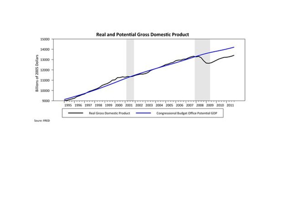


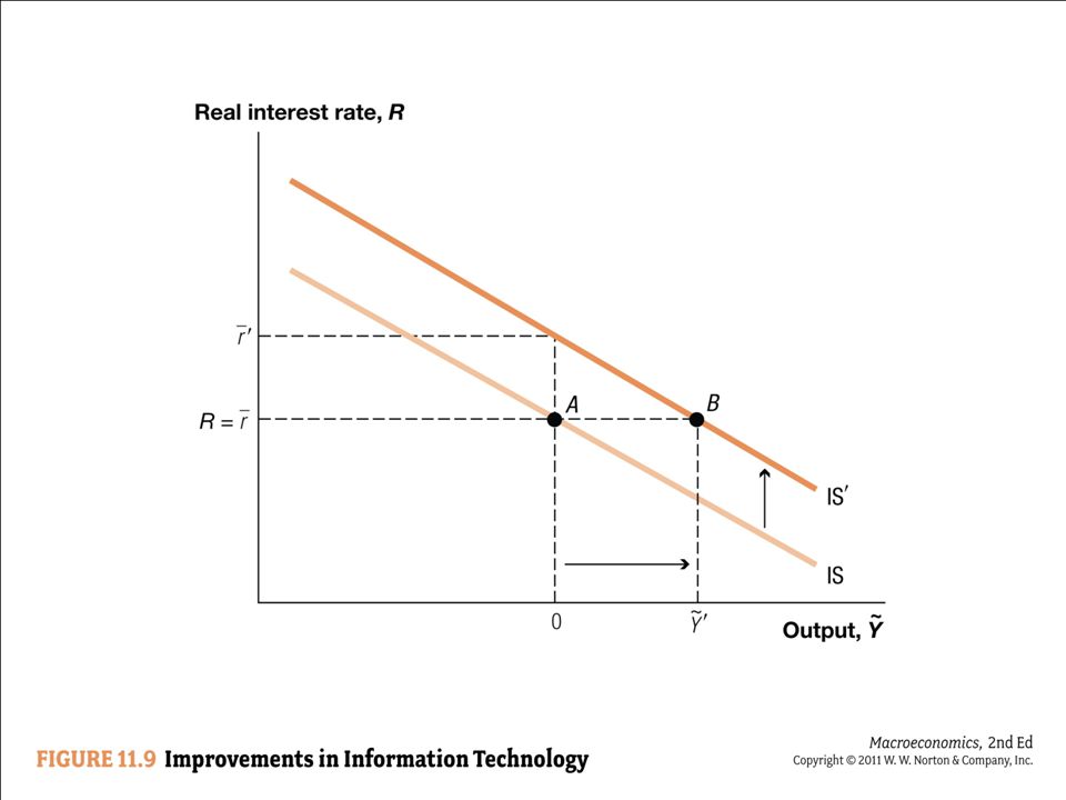

 to Asset Market (MP):>")


