Download presentation
Presentation is loading. Please wait.

1
Basics of H ∞ Control PART #1 the Loop-Shaping/Mixed Sensitivity Approach (to Robust & Optimal Control) Leonidas Dritsas PhD ldri@otenet.gr Version of 08-April-2012 Timestamp 08-Apr-12 THANKS TO… Prof. Kostas Kyriakopoulos (NTUA CSL) Prof. Kostas Kyriakopoulos (NTUA CSL) Panos Marantos (PhD candidate) Panos Marantos (PhD candidate)
 Prof. Kostas Kyriakopoulos (NTUA CSL) Panos Marantos (PhD candidate) Panos Marantos (PhD candidate).")
2
Note An H∞ “Crash Course” divides naturally into (at least) 3 parts: 1. Intro / Nominal Stability + Perform. / Freq. Domain (mainly) - Loopshaping – Mixed Sensitivity – Riccati Approach (DGKF’89) 2. ROBUST Stability + ROBUST Performance + “μ”-SSV 3. Linear Matrix Inequality (LMI), Bounded Real Lemma (BRL), Dissipativity, LMIreg, LPV + Gain Scheduling, Nonlinearities THIS PRESENTATION IS AN ATTEMPT FOR PART #1 !
 - Loopshaping – Mixed Sensitivity – Riccati Approach (DGKF’89) 2. ROBUST Stability + ROBUST Performance + μ -SSV 3. Linear Matrix Inequality (LMI), Bounded Real Lemma (BRL), Dissipativity, LMIreg, LPV + Gain Scheduling, Nonlinearities THIS PRESENTATION IS AN ATTEMPT FOR PART #1 !.")
3
Contents 1. Intro – Classical Feedback Control (internal) stability + performance + robustness (internal) stability + performance + robustness 2. SVD – Norms – {H ∞, H 2 } spaces & concepts in Control – the Engineering Interpratation 3. (Nominal) Controller Design 3.1 Loopshaping 3.2 Mixed Sensitivity (1-DOF architecture) 3.3 Generalized Plant + LFT 3.4 WHAT do the 3 filters represent ? 3.5 HOW do we select them? Fundamental Limitations in Control 4. MATLAB commands + examples (mixsyn/hinfsyn) 5. What’s next ? {“μ”-SSV, LMIs, BRL, dissipativity, LMIreg, LPV + Gain Scheduling, Nonlinearities} Αλέξης Παπαχαραλαμπόπουλος – Διπλωματική Εργασία 3/60
 stability + performance + robustness (internal) stability + performance + robustness 2. SVD – Norms – {H ∞, H 2 } spaces & concepts in Control – the Engineering Interpratation 3. (Nominal) Controller Design 3.1 Loopshaping 3.2 Mixed Sensitivity (1-DOF architecture) 3.3 Generalized Plant + LFT 3.4 WHAT do the 3 filters represent HOW do we select them. Fundamental Limitations in Control 4. MATLAB commands + examples (mixsyn/hinfsyn) 5. What’s next . { μ -SSV, LMIs, BRL, dissipativity, LMIreg, LPV + Gain Scheduling, Nonlinearities} Αλέξης Παπαχαραλαμπόπουλος – Διπλωματική Εργασία 3/60.")
4
http://www.nt.ntnu.no/users/skoge/book/

5
The Classical (1-DOF) Control Loop
 Control Loop")
6
The “Gang of Four” The “Gang of Four”: For internal stability must “check-stab” Four TFs

7
Two Degrees of Freedom Use a “prefilter” to meet both regulator and tracking performance The Gang of Six For internal stability must “check- stab” SIX TFs

8
Two Degrees of Freedom Alternative config.

10
1-DOF feedback control system Closed-loop response Control error : Plant input:

11
Design TRADE OFFs = “CANNOT HAVE IT ALL”

12
Closed-loop Performance Closed-loop Robustness Bode / Nyquist plots of L(jω)
")
13
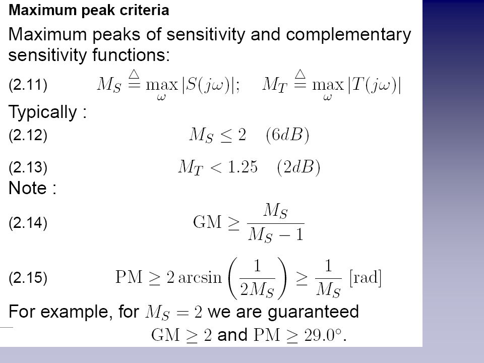
Max. (Peak) Sensitivity Ms
 Sensitivity Ms")
17
Controller design = TRADE OFFs = “CANNOT HAVE IT ALL”

20
Contents 1. Intro – Classical Feedback Control - (internal) stability + performance + robustness 2. SVD – Norms – {H ∞, H 2 } spaces & concepts in Control – the Engineering Interpratation 3. (Nominal) Controller Design 3.1 Loopshaping 3.2 Mixed Sensitivity (1-DOF architecture) 3.3 Generalized Plant + LFT 3.4 WHAT do the 3 filters represent ? 3.5 HOW do we select them? Fundamental Limitations in Control 4. MATLAB commands + examples (mixsyn/hinfsyn) 5. What’s next ? {“μ”-SSV, LMIs, BRL, dissipativity, LMIreg, LPV + Gain Scheduling, Nonlinearities} Αλέξης Παπαχαραλαμπόπουλος – Διπλωματική Εργασία 20/60
 Controller Design 3.1 Loopshaping 3.2 Mixed Sensitivity (1-DOF architecture) 3.3 Generalized Plant + LFT 3.4 WHAT do the 3 filters represent HOW do we select them. Fundamental Limitations in Control 4. MATLAB commands + examples (mixsyn/hinfsyn) 5. What’s next . { μ -SSV, LMIs, BRL, dissipativity, LMIreg, LPV + Gain Scheduling, Nonlinearities} Αλέξης Παπαχαραλαμπόπουλος – Διπλωματική Εργασία 20/60.")
22
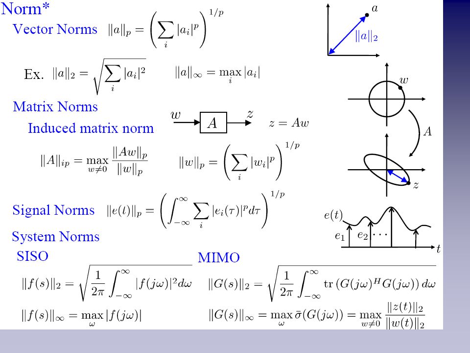
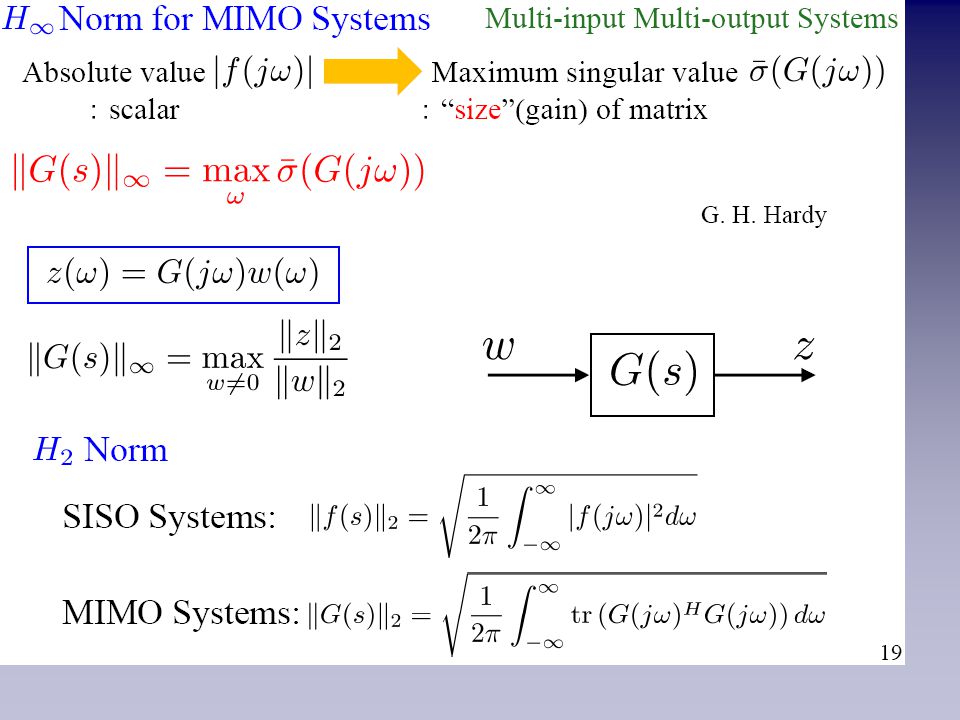
Signal & System Norms

23
Vector & Matrix Norm(s)
")
24
(Induced) Matrix Norms Vector & Matrix Norm(s)
 Matrix Norms Vector & Matrix Norm(s)")
28
Signal & System Norms

32
A paradigm shift: Generic control configuration (John Doyle) The concept of Generalized Plant Will be explained shortly
 The concept of Generalized Plant Will be explained shortly")
34
Contents 1. Intro – Classical Feedback Control - (internal) stability + performance + robustness 2. SVD – Norms – {H ∞, H 2 } spaces & concepts in Control – the Engineering Interpratation 3. (Nominal) Controller Design 3.1 Loopshaping 3.2 Mixed Sensitivity (1-DOF architecture) 3.3 Generalized Plant + LFT 3.4 WHAT do the 3 filters represent ? 3.5 HOW do we select them? Fundamental Limitations in Control 4. MATLAB commands + examples (mixsyn/hinfsyn) 5. What’s next ? {“μ”-SSV, LMIs, BRL, dissipativity, LMIreg, LPV + Gain Scheduling, Nonlinearities} 34/60
 Controller Design 3.1 Loopshaping 3.2 Mixed Sensitivity (1-DOF architecture) 3.3 Generalized Plant + LFT 3.4 WHAT do the 3 filters represent HOW do we select them. Fundamental Limitations in Control 4. MATLAB commands + examples (mixsyn/hinfsyn) 5. What’s next . { μ -SSV, LMIs, BRL, dissipativity, LMIreg, LPV + Gain Scheduling, Nonlinearities} 34/60.")
35
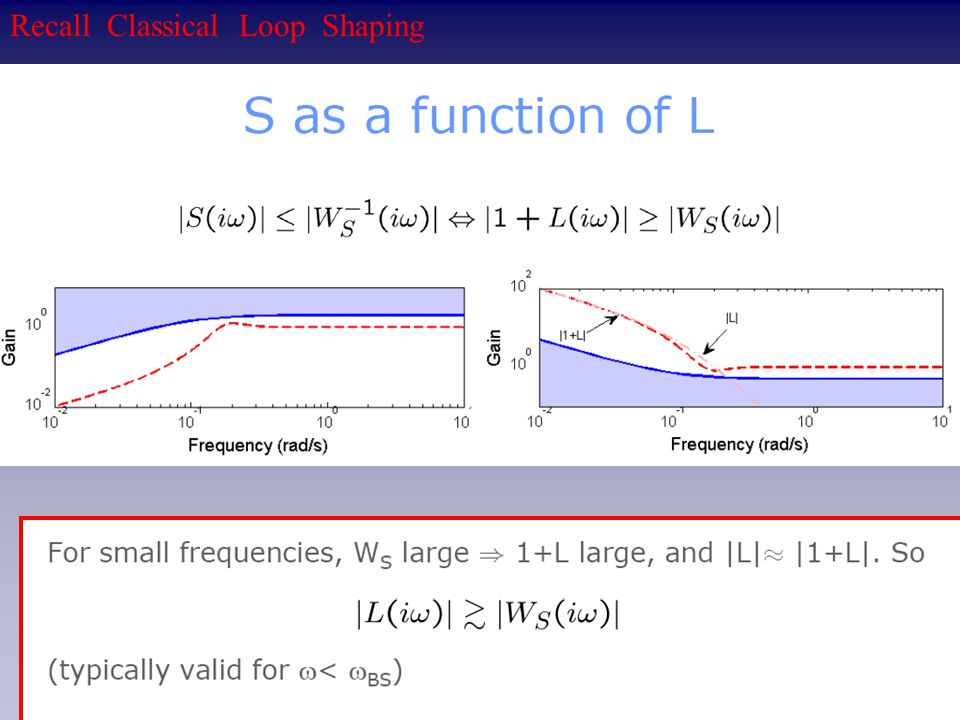
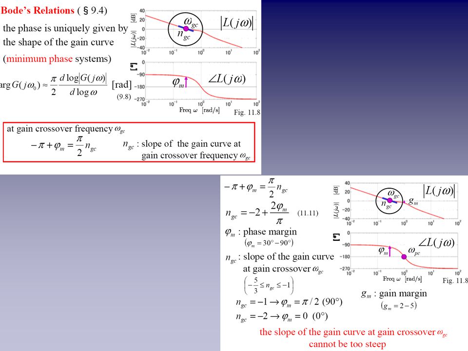
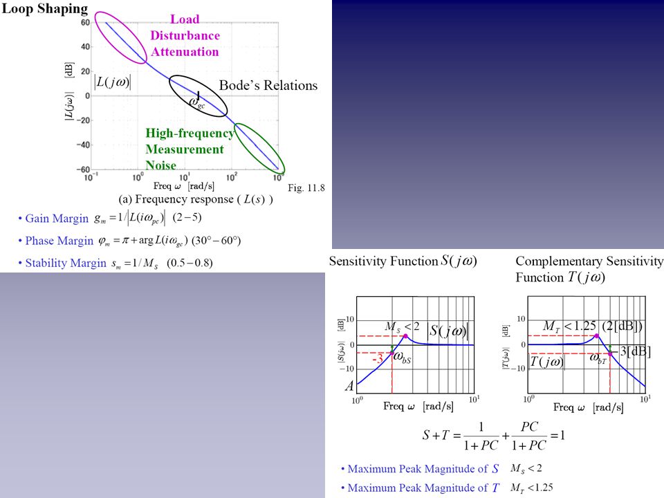
Recall Classical Loop Shaping

38
Recall Classical Loop Shaping - Relation to stability margins

45
Contents 1. Intro – Classical Feedback Control - (internal) stability + performance + robustness 2. SVD – Norms – {H ∞, H 2 } spaces & concepts in Control – the Engineering Interpratation 3. (Nominal) Controller Design 3.1 Loopshaping 3.2 Mixed Sensitivity (1-DOF architecture) 3.3 Generalized Plant + LFT 3.4 WHAT do the 3 filters represent ? 3.5 HOW do we select them? Fundamental Limitations in Control 4. MATLAB commands + examples (mixsyn/hinfsyn) 5. What’s next ? {“μ”-SSV, LMIs, BRL, dissipativity, LMIreg, LPV + Gain Scheduling, Nonlinearities} 45/60
 Controller Design 3.1 Loopshaping 3.2 Mixed Sensitivity (1-DOF architecture) 3.3 Generalized Plant + LFT 3.4 WHAT do the 3 filters represent HOW do we select them. Fundamental Limitations in Control 4. MATLAB commands + examples (mixsyn/hinfsyn) 5. What’s next . { μ -SSV, LMIs, BRL, dissipativity, LMIreg, LPV + Gain Scheduling, Nonlinearities} 45/60.")
57
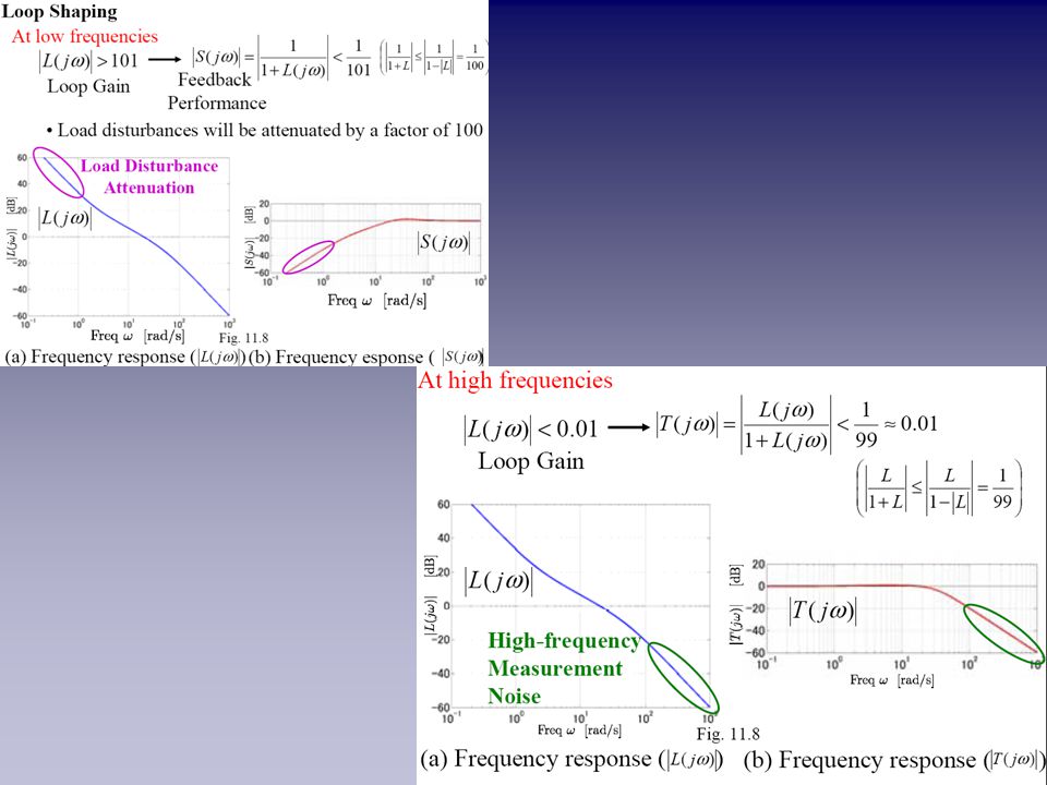
Loop gain specifications S as a function of L

58
T as a function of L Relation to stability margins

59
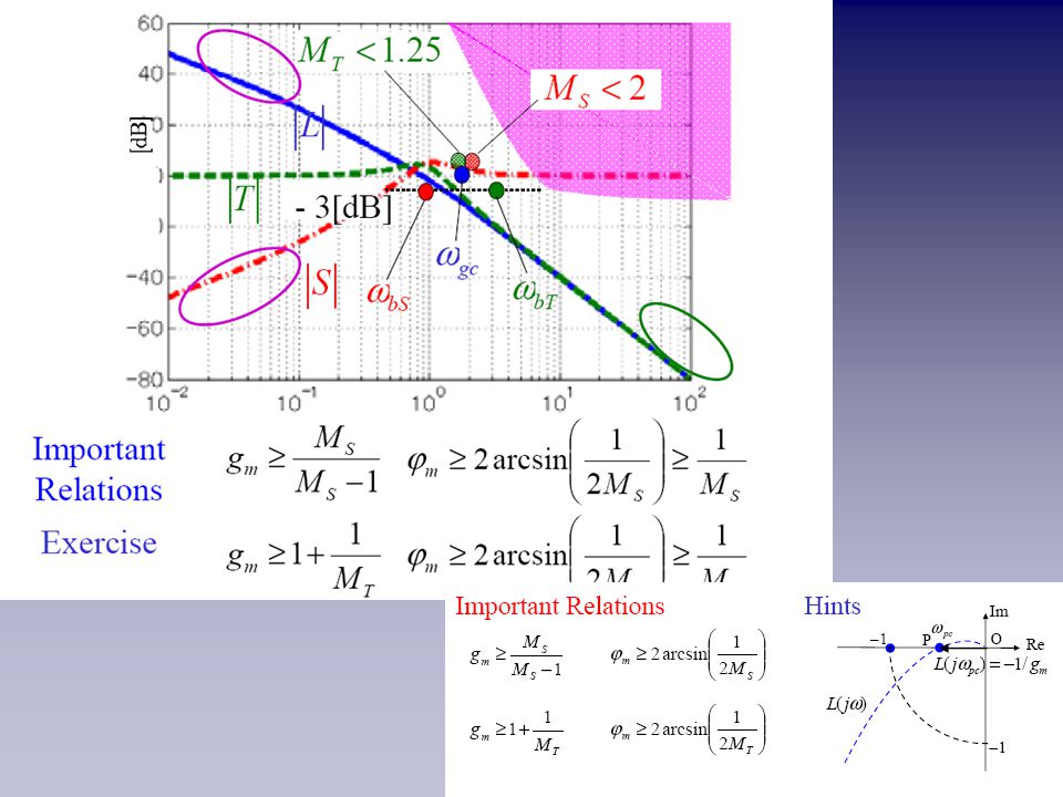
Probably the most important slide (for Design purposes) Same as slide #44
 Same as slide #44")
60
Probably the most important slide (for Design purposes)
")
63
Contents 1. Intro – Classical Feedback Control (internal) stability + performance + robustness (internal) stability + performance + robustness 2. SVD – Norms – H∞ - H 2 - Engineering Interpr. 3. (Nominal) Controller Design Loopshaping – Mixed Sensitivity (1-DOF architecture) Loopshaping – Mixed Sensitivity (1-DOF architecture) Generalized Plant + LFT Generalized Plant + LFT WHAT do the 3 filters represent ? WHAT do the 3 filters represent ? HOW do we select the 3 filters ? Fundamental Limitations HOW do we select the 3 filters ? Fundamental Limitations 4. MATLAB commands + examples (mixsyn/hinfsyn)
 stability + performance + robustness (internal) stability + performance + robustness 2. SVD – Norms – H∞ - H 2 - Engineering Interpr. 3. (Nominal) Controller Design Loopshaping – Mixed Sensitivity (1-DOF architecture) Loopshaping – Mixed Sensitivity (1-DOF architecture) Generalized Plant + LFT Generalized Plant + LFT WHAT do the 3 filters represent . WHAT do the 3 filters represent . HOW do we select the 3 filters . Fundamental Limitations HOW do we select the 3 filters . Fundamental Limitations 4. MATLAB commands + examples (mixsyn/hinfsyn).")
65
Separate Lecture on Robustness

66
The SMALL GAIN Theorem

67
Robustness Interpretation of W1, W2, W3 filters

69
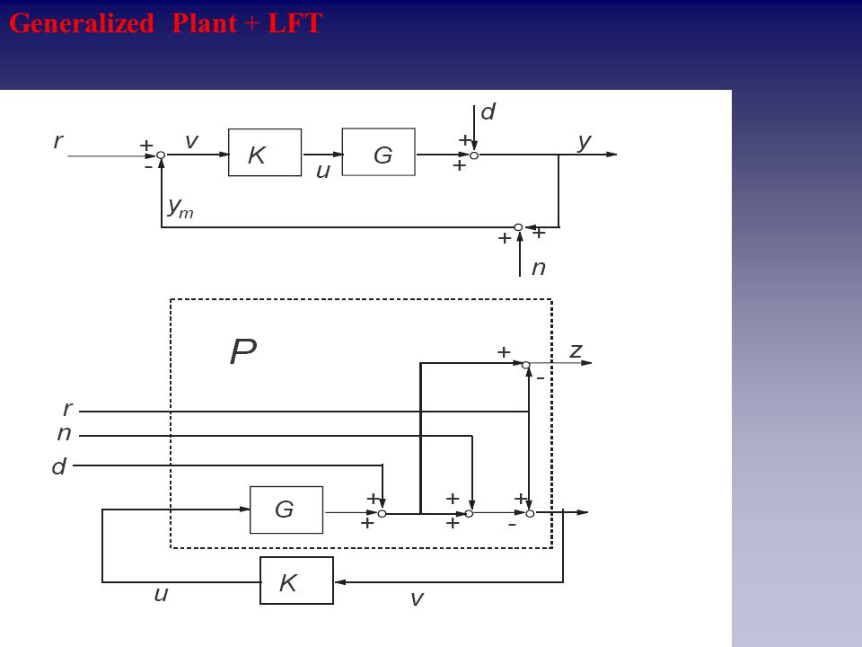
Generalized Plant + LFT

73
Generalized Plant for the Classical Control Loop

74
Standard Problem: P-K-Structure + LFT = Linear Fractional Transformations (Upper & Lower)
")
75
LFT = Linear Fractional Transformations (Upper & Lower)
")
76
Contents 1. Intro – Classical Feedback Control - (internal) stability + performance + robustness 2. SVD – Norms – {H ∞, H 2 } spaces & concepts in Control – the Engineering Interpratation 3. (Nominal) Controller Design 3.1 Loopshaping 3.2 Mixed Sensitivity (1-DOF architecture) 3.3 Generalized Plant + LFT 3.4 WHAT do the 3 filters represent ? 3.5 HOW do we select them? Fundamental Limitations in Control 4. MATLAB commands + examples (mixsyn/hinfsyn) 5. What’s next ? {“μ”-SSV, LMIs, BRL, dissipativity, LMIreg, LPV + Gain Scheduling, Nonlinearities} 76/60
 Controller Design 3.1 Loopshaping 3.2 Mixed Sensitivity (1-DOF architecture) 3.3 Generalized Plant + LFT 3.4 WHAT do the 3 filters represent HOW do we select them. Fundamental Limitations in Control 4. MATLAB commands + examples (mixsyn/hinfsyn) 5. What’s next . { μ -SSV, LMIs, BRL, dissipativity, LMIreg, LPV + Gain Scheduling, Nonlinearities} 76/60.")
77
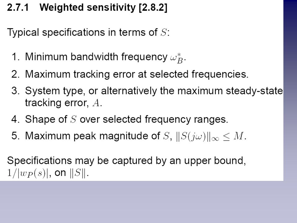
Fundamental Performance Limitations reflected in filter limitations 1. Perfect control & plant inversion

78
Fundamental Performance Limitations reflected in filter limitations 2 Constraints on S and T 3 The waterbed effects (BODE sensitivity integrals 1945) 4 Interpolation constraints from internal stability
 4 Interpolation constraints from internal stability")
79
Fundamental Performance Limitations reflected in filter limitations 5 Sensitivity peaks - Maximum modulus Principle.

80
Fundamental Performance Limitations reflected in filter limitations

81
Fundamental Performance Limitations reflected in filter limitations

82
Fundamental Performance Limitations reflected in filter limitations

83
Fundamental Performance Limitations reflected in filter limitations Limitations imposed by RHP- poles

84
Limiting factors

85
Contents 1. Intro – Classical Feedback Control - (internal) stability + performance + robustness 2. SVD – Norms – {H ∞, H 2 } spaces & concepts in Control – the Engineering Interpratation 3. (Nominal) Controller Design 3.1 Loopshaping 3.2 Mixed Sensitivity (1-DOF architecture) 3.3 Generalized Plant + LFT 3.4 WHAT do the 3 filters represent ? 3.5 HOW do we select them? Fundamental Limitations in Control 4. MATLAB commands + examples (mixsyn/hinfsyn) 5. What’s next ? {“μ”-SSV, LMIs, BRL, dissipativity, LMIreg, LPV + Gain Scheduling, Nonlinearities} 85/60
 Controller Design 3.1 Loopshaping 3.2 Mixed Sensitivity (1-DOF architecture) 3.3 Generalized Plant + LFT 3.4 WHAT do the 3 filters represent HOW do we select them. Fundamental Limitations in Control 4. MATLAB commands + examples (mixsyn/hinfsyn) 5. What’s next . { μ -SSV, LMIs, BRL, dissipativity, LMIreg, LPV + Gain Scheduling, Nonlinearities} 85/60.")
87
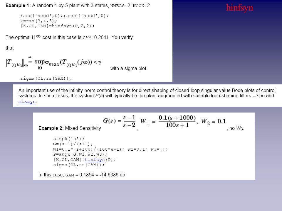
hinfsyn

89
mixsyn

92
Contents 1. Intro – Classical Feedback Control - (internal) stability + performance + robustness 2. SVD – Norms – {H ∞, H 2 } spaces & concepts in Control – the Engineering Interpratation 3. (Nominal) Controller Design 3.1 Loopshaping 3.2 Mixed Sensitivity (1-DOF architecture) 3.3 Generalized Plant + LFT 3.4 WHAT do the 3 filters represent ? 3.5 HOW do we select them? Fundamental Limitations in Control 4. MATLAB commands + examples (mixsyn/hinfsyn) 5. What’s next ? “μ”-SSV, LMIs, BRL, dissipativity, “LMIreg”, LPV + Gain Scheduling, Handling Nonlinearities 92/60
 Controller Design 3.1 Loopshaping 3.2 Mixed Sensitivity (1-DOF architecture) 3.3 Generalized Plant + LFT 3.4 WHAT do the 3 filters represent HOW do we select them. Fundamental Limitations in Control 4. MATLAB commands + examples (mixsyn/hinfsyn) 5. What’s next . μ -SSV, LMIs, BRL, dissipativity, LMIreg , LPV + Gain Scheduling, Handling Nonlinearities 92/60.")
93
THANK YOU FOR YOUR ATTENTION THE END THANK YOU FOR YOUR ATTENTION THANKS TO… Prof. Kostas Kyriakopoulos (NTUA CSL) Prof. Kostas Kyriakopoulos (NTUA CSL) Panos Marantos (PhD candidate) Panos Marantos (PhD candidate)
 Prof. Kostas Kyriakopoulos (NTUA CSL) Panos Marantos (PhD candidate) Panos Marantos (PhD candidate).")
96
Contents 1. Intro – Classical Feedback Control - (internal) stability + performance + robustness 2. SVD – Norms – {H ∞, H 2 } spaces & concepts in Control – the Engineering Interpratation 3. (Nominal) Controller Design 3.1 Loopshaping 3.2 Mixed Sensitivity (1-DOF architecture) 3.3 Generalized Plant + LFT 3.4 WHAT do the 3 filters represent ? 3.5 HOW do we select them? Fundamental Limitations in Control 4. MATLAB commands + examples (mixsyn/hinfsyn) 5. What’s next ? {“μ”-SSV, LMIs, BRL, dissipativity, LMIreg, LPV + Gain Scheduling, Nonlinearities} 96/60
 Controller Design 3.1 Loopshaping 3.2 Mixed Sensitivity (1-DOF architecture) 3.3 Generalized Plant + LFT 3.4 WHAT do the 3 filters represent HOW do we select them. Fundamental Limitations in Control 4. MATLAB commands + examples (mixsyn/hinfsyn) 5. What’s next . { μ -SSV, LMIs, BRL, dissipativity, LMIreg, LPV + Gain Scheduling, Nonlinearities} 96/60.")
97
Contents 1. Intro – Classical Feedback Control (internal) stability + performance + robustness (internal) stability + performance + robustness 2. SVD – Norms – H∞ - H 2 - Engineering Interpr. 3. (Nominal) Controller Design Loopshaping – Mixed Sensitivity (1-DOF architecture) Loopshaping – Mixed Sensitivity (1-DOF architecture) WHAT do the 3 filters represent ? WHAT do the 3 filters represent ? HOW do we select the 3 filters ? Fundamental Limitations HOW do we select the 3 filters ? Fundamental Limitations 4. MATLAB commands + examples (mixsyn/hinfsyn) 5. What’s next ? “μ”-SSV, LMIs, BRL, dissipativity, LMIreg, LPV + Gain Scheduling, Nonlinearities
 stability + performance + robustness (internal) stability + performance + robustness 2. SVD – Norms – H∞ - H 2 - Engineering Interpr. 3. (Nominal) Controller Design Loopshaping – Mixed Sensitivity (1-DOF architecture) Loopshaping – Mixed Sensitivity (1-DOF architecture) WHAT do the 3 filters represent . WHAT do the 3 filters represent . HOW do we select the 3 filters . Fundamental Limitations HOW do we select the 3 filters . Fundamental Limitations 4. MATLAB commands + examples (mixsyn/hinfsyn) 5. What’s next . μ -SSV, LMIs, BRL, dissipativity, LMIreg, LPV + Gain Scheduling, Nonlinearities.")
100
Modeling for “small” ( k < h) and “Long” delays Modeling for “small” ( τ k < h) and “Long” delays
 and Long delays Modeling for small ( τ k < h) and Long delays")
Similar presentations


 0db.>")


