1. Chapter 10 Stability Analysis and Controller Tuning
※ Bounded-input bounded-output (BIBO) stability
＊ Ex A level process with P control

2. (S1) Models
(S2) Solution by Laplace transform
where

3. Note:
Stable if Kc<0
Unstable Kc>0
Steady state performance by

4. ＊ Ex. 10.3 A level process without control
Response to a sine flow disturbance
Response to a step flow disturbance

5. ※ Stability analysis

6. Note: Assume Gd(s) is stable.

7. ＊ Stability of linearized closed-loop systems
Ex The series chemical reactors with PI controller

8. @ Known values
Process
Controller

9. @ Formulation& stability
Stable

10. ◎ Criterion of stability
※ Direct substitution method

11. The response of controlled output:

12. P3.

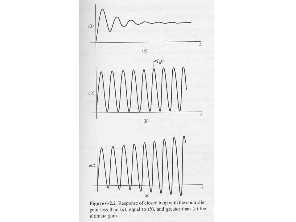
13. ﹪Ultimate gain (Kcu): The controller gain at which this point of marginal instability is reached
﹪Ultimate period (Tu): It shows the period of the oscillation at the ultimate gain
＊ Using the direct substitution method by in the characteristic equation

15. Example A.1 Known transfer functions

16. Find: (1) Ultimate gain
(2) Ultimate period
S1. Characteristic eqn.

17. S2. Let at Kc=Kcu

19. Example A.2
S1.

20. S2.
S3.

21. Example A.3 Find the following control loop: (1) Ultimate gain
(2) Ultimate period

22. S1. The characteristic eqn. for H(s)=KT/(Ts+1)
S2. Gc=-Kc to avoid the negative gains in the characteristic eqn.

23. S3. By direct substitution of at Kc=Kcu

24. ＊ Dead-time
Since the direct substitution method fails when any of blocks
on the loop contains deadt-ime term, an approximation to the
dead-time transfer function is used.
First-order Padé approximation:

25. Example A.4 Find the ultimate gain and frequency of first-order plus dead-time process
S1. Closed-loop system with P control

26. S2. Using Pade approximation

27. S3. Using direct substitution method

28. Note:
The ultimate gain goes to infinite as the dead-time approach zero.
The ultimate frequency increases as the dead time decreases.

29. ※ Root locus
A graphical technique consists of roots of characteristic equation and control loop parameter changes.

30. ＊Definition:
Characteristic equation:
Open-loop transfer function (OLTF):
Generalized OLTF:

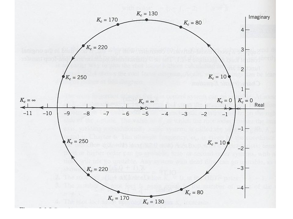
31. Example B.1: a characteristic equation is given
S1. Decide open-loop poles and zeros by OLTF

32. S2. Depict by the polynomial (characteristic equation)
Kc:1/3

33. S3. Analysis

34. Example B.2: a characteristic equation is given
S1. Decide poles and zeros

35. S2. Depict by the polynomial (characteristic equation)

36. S3. Analysis

37. Example B.3: a characteristic equation is given
S1. Decide poles and zeros
S2. Depict by the polynomial (characteristic equation)

39. S3. Analysis

40. @ Review of complex number
c=a+ib

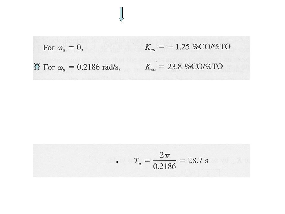
41. Polar notations

42. P1. Multiplication for two complex numbers (c, p)
P2. Division for two complex numbers (c, p)

43. @ Rules for root locus diagram
Characteristic equation
Magnitude and angle conditions

44. Since

45. Rule for searching roots of characteristic equation
Ex. A system have two OLTF poles (x) and one OLTF zero (o)
Note: If the angle condition is satisfied, then the point s1 is the part of the root locus

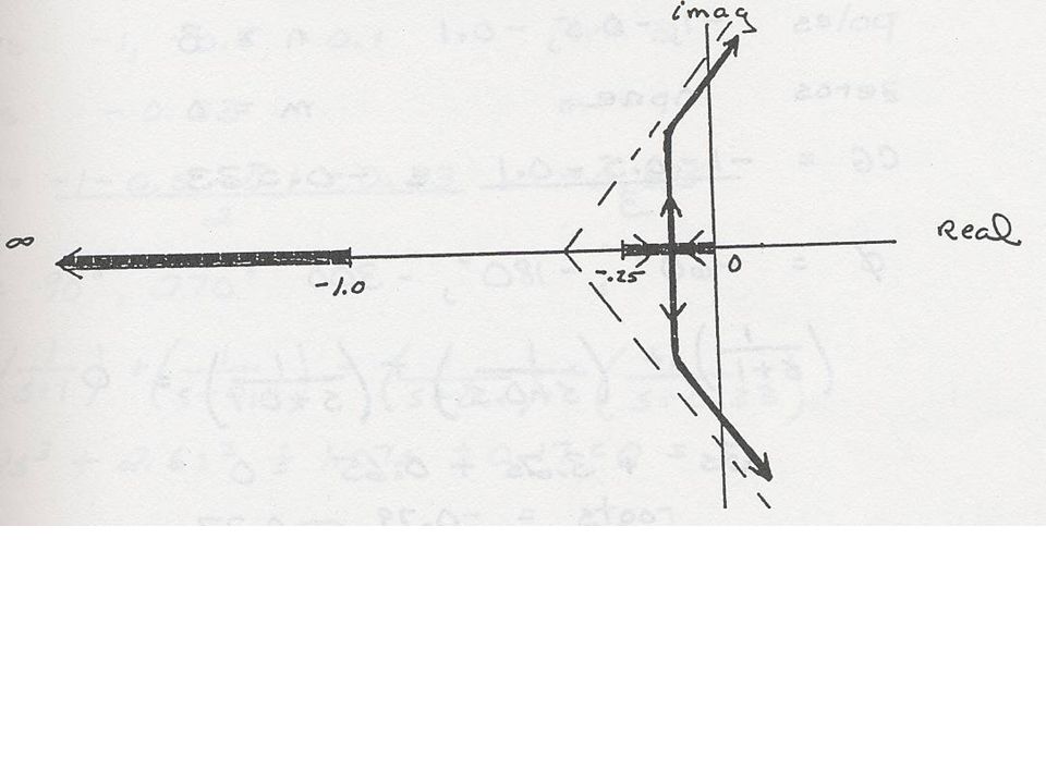
48. Example B.4 Depict the root locus of a characteristic equation (heat exchanger control loop with P control)
S1. OLTF

49. S2. Rule for root locus
From rule 1 where the root locus exists are indicated.
From rule 2 indicate that the root locus is originated at the poles of OLTF.
n=3, three branches or loci are indicated.
Because m=0 (zeros), all loci approach infinity as Kc increases.
Determine CG= and asymptotes with angles, =60°, 180 °, 300 °.
Calculate the breakaway point by

50. s= – and –0.063
S3. Depict the possible root locus with ωu=0.22 (direct substitution method) and Kcu=24

51. Example B.5 Depict the root locus of a characteristic equation (heat exchanger control loop with PI control)
S1. OLTF

52. S2. Following rules

53. S3. Depict root locus

54. ＊Exercises

55. Ans. 8.1

57. Ans. 8.2

61. ＊ Dynamic responses for various pole locations

62. ＊ Which is good method for stability analysis◎

63. ※ Bode method
A brief review:
OLTF
Frequency response

64. ◎ Stability criterion

66. ＊ Frequency response stability criterion
Determining the frequency at which the phase angle of OLTF is –180°(–π) and AR of OLTF at that frequency
Ex. C.1 Heat exchanger control system (Ex. A.1)

67. S1. OLTF
S2. Find MR and θ
S3. Bode plot in Fig to estimate ω=0.219 by θ= –180°
and decide MR=0.0524

69. S4. Decide Kc as AR=1 ＃
＊ Stability vs. controller gain
In Bode plot, as θ= –180° both ω and MR are determined. Moreover, ω = ωu and Kcu can be obtained.

70. Ex. C.2 Analysis of stability for a OTLF
S1. MR and θ

71. S2. Show Bode plot
(MR vs.  &  vs.  )

72. S3. Find ωu and Kcu
ωu=0.16 by = –π
Kcu =12.8
Ex. C.3 The same process with PD controller
and =0.1
(S1) OLTF

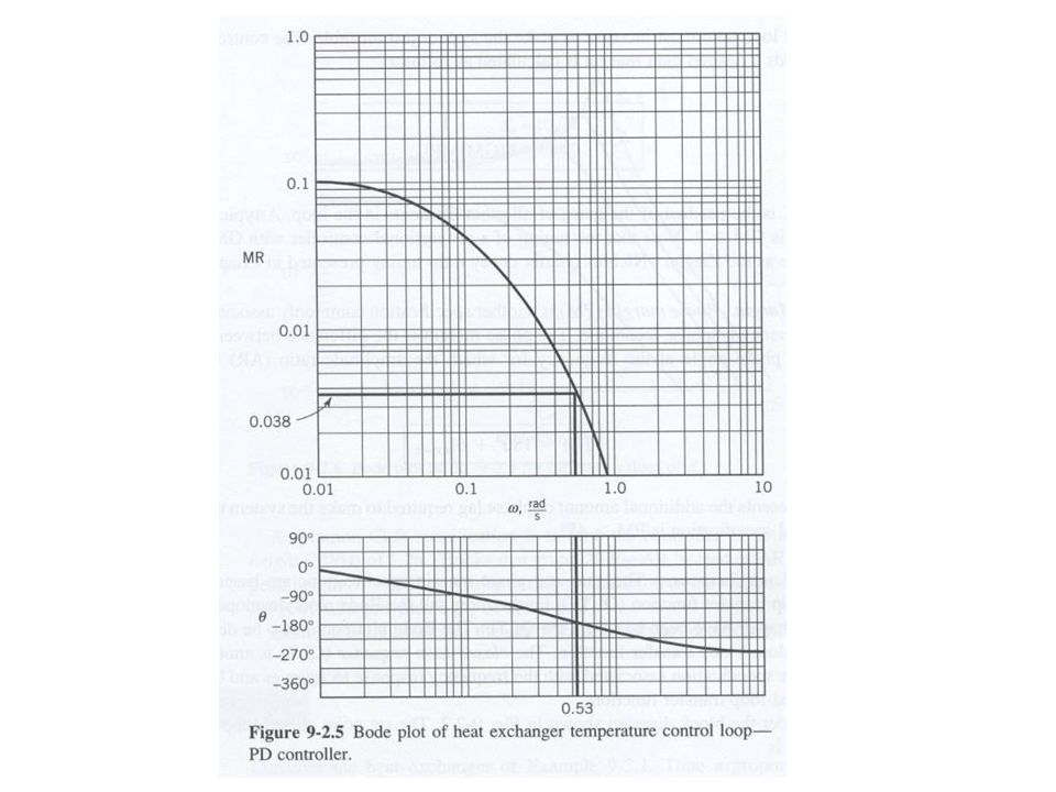
73. (S2) By Fig
u=0.53 and MR=0.038
Kcu=33 and u=0.53

75. Ex. 10.7
(S1) Bode plot (AR vs.  &  vs.  ) for Kc=1

76. (S2) Stability vs. controller gain Kc
Ex Determine whether this system is stable.

77. (S1) Bode plot for Kc=15 and TI=1
(S2) Since the AR>1 at , the system is unstable.

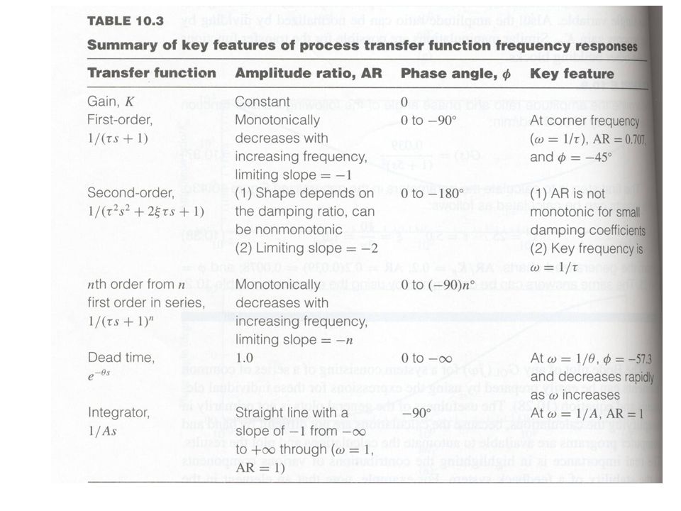
78. P1. Bode plot for the first-order system

79. P2. Bode plot for the second-order system

80. Ex. 10.9 Determine AR and  of the following transfer function at

82. ＊ Controller tuning based on Z-N closed-loop tuning method
S1. Calculating c by setting Kc=1
and then determine Ku and Pu
where ARc=

83. S2. Controller tuning constants
Ex Calculate controller tuning constants for a process, Gp(s)=0039/(5s+1)3, by uning the Z-N method
S1.

84. S2. Bode plot

85. S3. Tuning constants

86. S4. Closed-loop test

87. Ex. 10.14 Integral mode tend to destabilize the control system

88. @ Effect of modeling errors on stability
Gain margin (GM): Total loop gain increase to make the system
just unstable. The controller gain that yields a gain margin
＊ Typical specification: GM2
If P controller with GM=2 is the same as the Z-N tuning.

89. (2) Phase margin (PM):
＊ Typical specification: PM>45°
Ex. D.1 Consider the same heat exchanger to tune a P controller for specifications (Ex. C.2)
(a) While GM=2

90. (b) PM= 45°θ= –135°. By Fig. in Ex. C.2, we can find
and

91. ※ Polar plot
The polar plot is a graph of the complex-valued function G(i)
as  goes from 0 to .
Ex. E.1 Consider the amplitude ratio and the phase angle angle of
first-order lag are given as

93. Ex. E.2 Consider the amplitude ratio and the phase angle angle of
second-order lag are given as

95. Ex. E.3 Consider the second-order system with tuning Kc

96. Ex. E.4. Consider the amplitude ratio and the phase angle angle of
pure dead time system are given as

97. ※ Conformal mapping

98. ※ Nyquist stability criterion (Nyquist plot)
Ex. E.5 Consider a closed-loop system, its OLTF is given as

100. Unstable stable
Kc>23.8
Marginal stable
Kc=23.8
stable
Kc<23.8

101. Exercises:
Q.10.11
Q.10.15