1. Graph Visualization

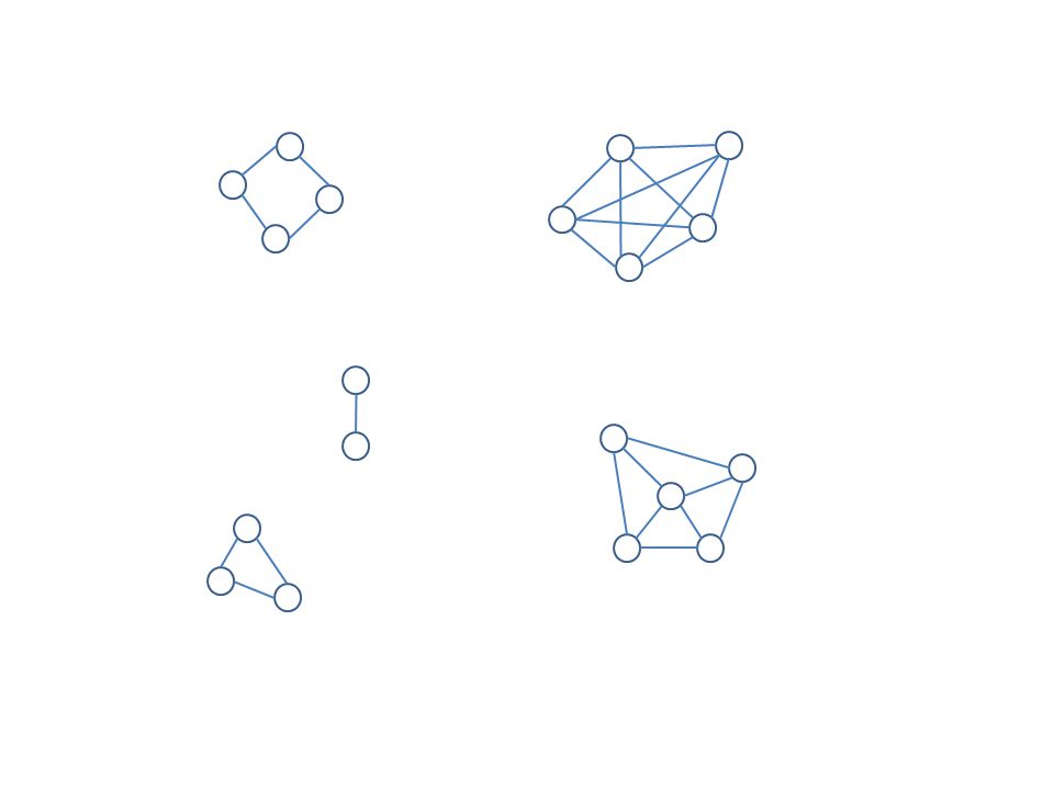
2. What is a Graph 2 1 4 5 3 6 2 1 4 5 3 6

3. Graphs are everywhere

4. Basic Concepts

5. Image source: http://people.seas.harvard.edu/~joshlee/ Image source: http://www.sagemath.org/doc/thematic_tutorials/linear_progra mming.html/

6. 12 34 56 78 3-D 12 34 56 78 planar

7. Basic Concepts

9. Basic Concepts (II) 2 1 4 5 3 6 7 8 9 2 1 4 5 3 6 7 8 9

10. – The length of the path is the number of edges on it – The distance between two nodes is the shortest path connecting them. – A graph is connected if there exist paths between all pairs of vertices; otherwise, it is disconnected. – The minimum number of edges that would need to be removed from G in order to make the graph disconnected is the edge- connectivity of the graph. 2 1 4 5 3 6 7 8 9 2 1 4 5 3 6 7 8 9

11. Basic Concepts (III) – A cycle is a simple path that begins and ends at the same vertex. – A graph that contains on cycle is acyclic and is also called forest. – A connected forest is called a tree. 2 1 4 5 3 6 7 8 9 2 1 4 5 3 6 7 8 9

12. Basic Concepts (IV) 2 1 4 5 3 6 7 8 9

13. http://www.i-cherubini.it/mauro/blog/2006/04/06/minimum-spanning-tree-of- urban-tapestries-messages/

14. Basic Graph Layout Techniques Force-direct layout Arc-diagram Adjacent matrix Circular layout

15. Basic Graph Layout Techniques Force-direct layout Arc-diagram Adjacent matrix Circular layout

16. Force-Direct Layout of Graph We already know: – The most common graphical representation of a network is a node-link diagram, where each node is shown as a point, circle, polygon, or some other small graphical object, and each edge is shown as a line segment or curve connecting two nodes. Force-Direct Layout idea: – We imagine the nodes as physical particles that are initialized with random positions, but are gradually displaced under the effect of various forces, until they arrive at a final position. The forces are defined by the chosen algorithm, and typically seek to position adjacent nodes near each other, but not too near.

17. Force-Direct Layout of Graph

18. Implementation – To implement this force-directed layout, assume that the nodes are stored in an array nodes[], where each element of the array contains a position x, y and the net force force_x, force_y acting on the node. – The forces are simulated in a loop that computes the net forces at each time step and updates the positions of the nodes, hopefully until the layout converges to some good distributed positions.

19. Force-Direct Layout of Graph 1 L =... // spring rest length 2 K_r =... // repulsive force constant 3 K_s =... // spring constant 4 delta_t =... // time step 5 6 N = nodes.length 7 8 // initialize net forces 9 for i = 0 to N-1 10 nodes[i].force_x = 0 11 nodes[i].force_y = 0 12 13 // repulsion between all pairs 14 for i1 = 0 to N-2 15 node1 = nodes[i1] 16 for i2 = i1+1 to N-1 17 node2 = nodes[i2] 18 dx = node2.x - node1.x 19 dy = node2.y - node1.y 20 if dx != 0 or dy != 0 21 distanceSquared = dx *dx + dy*dy 22 distance = sqrt( distanceSquared ) 23 force = K_r / distanceSquared 24 fx = force * dx / distance 25 fy = force * dy / distance 26 node1.force_x = node1.force_x - fx 27 node1.force_y = node1.force_y - fy 28 node2.force_x = node2.force_x + fx 29 node2.force_y = node2.force_y + fy 30 31 // spring force between adjacent pairs 32 for i1 = 0 to N-1 33 node1 = nodes[i1] 34 for j = 0 to node1.neighbors.length-1 35 i2 = node1.neighbors[j] 36 node2 = nodes[i2] 37 if i1 < i2 38 dx = node2.x - node1.x 39 dy = node2.y - node1.y 40 if dx != 0 or dy != 0 41 distance = sqrt( dx*dx + dy*dy ) 42 force = K_s*( distance - L ) 43 fx = force*dx / distance 44 fy = force*dy / distance 45 node1.force_x = node1.force_x + fx 46 node1.force_y = node1.force_y + fy 47 node2.force_x = node2.force_x - fx 48 node2.force_y = node2.force_y - fy 49 50 // update positions 51 for i = 0 to N-1 52 node = nodes[i] 53 dx = delta_t*node.force_x 54 dy = delta_t*node.force_y 55 displacementSquared = dx*dx + dy*dy 56 if ( displacementSquared > MAX_DISPLACEMENT_SQUARED ) 57 s = sqrt( MAX_DISPLACEMENT_SQUARED / displacementSquared ) 58 dx = dx *s 59 dy = dy*s 60 node.x = node.x + dx 61 node.y = node.y + dy

20. Force-Direct Layout of Graph 1 L =... // spring rest length 2 K_r =... // repulsive force constant 3 K_s =... // spring constant 4 delta_t =... // time step 5 6 N = nodes.length 7 8 // initialize net forces 9 for i = 0 to N-1 10 nodes[i].force_x = 0 11 nodes[i].force_y = 0 12 13 // repulsion between all pairs 14 for i1 = 0 to N-2 15 node1 = nodes[i1] 16 for i2 = i1+1 to N-1 17 node2 = nodes[i2] 18 dx = node2.x - node1.x 19 dy = node2.y - node1.y 20 if dx != 0 or dy != 0 21 distanceSquared = dx *dx + dy*dy 22 distance = sqrt( distanceSquared ) 23 force = K_r / distanceSquared 24 fx = force * dx / distance 25 fy = force * dy / distance 26 node1.force_x = node1.force_x - fx 27 node1.force_y = node1.force_y - fy 28 node2.force_x = node2.force_x + fx 29 node2.force_y = node2.force_y + fy 30 31 // spring force between adjacent pairs 32 for i1 = 0 to N-1 33 node1 = nodes[i1] 34 for j = 0 to node1.neighbors.length-1 35 i2 = node1.neighbors[j] 36 node2 = nodes[i2] 37 if i1 < i2 38 dx = node2.x - node1.x 39 dy = node2.y - node1.y 40 if dx != 0 or dy != 0 41 distance = sqrt( dx*dx + dy*dy ) 42 force = K_s*( distance - L ) 43 fx = force*dx / distance 44 fy = force*dy / distance 45 node1.force_x = node1.force_x + fx 46 node1.force_y = node1.force_y + fy 47 node2.force_x = node2.force_x - fx 48 node2.force_y = node2.force_y - fy 49 50 // update positions 51 for i = 0 to N-1 52 node = nodes[i] 53 dx = delta_t*node.force_x 54 dy = delta_t*node.force_y 55 displacementSquared = dx*dx + dy*dy 56 if ( displacementSquared > MAX_DISPLACEMENT_SQUARED ) 57 s = sqrt( MAX_DISPLACEMENT_SQUARED / displacementSquared ) 58 dx = dx *s 59 dy = dy*s 60 node.x = node.x + dx 61 node.y = node.y + dy

21. Force-Direct Layout of Graph Force-directed node-link diagrams of a 43-node, 80-edge network. Left: a low spring constant makes the edges more flexible. Right: a high spring constant makes them more stiff

22. Force-Direct Layout of Graph Limitations and Improvements – Difficult to choose a proper delta_t :If the time step delta_t (used at lines 53, 54) is too small, many iterations will be needed to converge. On the other hand, if the time step is too large, or if the net forces generated are too large, the positions of nodes may oscillate and never converge. Line 56 imposes a limit on such movement. – As a minor optimization, line 56 compares squares (i.e., displacementSquared>MAX_DISPLACEMENT_SQUARED rather than displacement >MAX_DISPLACEMENT), to avoid the cost of computing a square root (unless the if succeeds)

23. Force-Direct Layout of Graph Limitations and Improvements – The GEM[16] algorithm speeds up convergence by decreasing a “temperature” parameter as the layout progresses, allowing nodes to move larger distances earlier in the process, and then constraining their movements progressively toward the end.

24. Force-Direct Layout of Graph Limitations and Improvements – A minor improvement to the above pseudocode would be to detect if the distance between two nodes is zero (by adding an else clause to the if statement at line 20), and in that case to generate a small force between the two nodes in some random direction, to push them apart. Without this, if the two nodes happen to have the same neighbors, they may remain forever “stuck” to each other.

25. Force-Direct Layout of Graph

27. Limitations and Improvements As can be seen in the left example, the multiple crossings of edges can make it unclear when certain edges pass close to a node or are connected to a node. Also, in such layouts where the nodes are rather closely packed, there isn’t much room left to display labels or other information associated with each node This leads to the next layout method Force-directed node-link diagram of a random 50-node, 200-edge graph.

28. Basic Graph Layout Techniques Force-direct layout Arc-diagram Adjacent matrix Circular layout

29. Arc Diagrams and Barycenter Ordering It is sometimes useful to layout the nodes of a network along a straight line, in what might be called linearization. With such a layout, edges can be drawn as circular arcs, yielding an arc diagram. It is important that the arcs in the diagram all cover the same angle, such as 180 degrees. This way, an arc between nodes n1 and n2 will extend outward by a distance proportional to the distance between n1 and n2, making it easier to disambiguate the arcs. Arc diagrams of a 43-node, 80-edge network

30. Arc Diagrams and Barycenter Ordering An arc covering angle θ, with center C

31. We might order the nodes to reduce the total length of the arcs, making the topology of the network easier to understand. Sorting the nodes: Arc Diagrams and Barycenter Ordering Left: with a random ordering and 180-degree arcs. Middle: after applying the barycenter heuristic to order the nodes. Right: after changing the angles of the arcs to 100 degrees.

32. We might order the nodes to reduce the total length of the arcs, making the topology of the network easier to understand. There are many algorithms for computing such an ordering. However, we will discuss an easy-to- program technique called the barycenter heuristic. Sorting the nodes: Arc Diagrams and Barycenter Ordering The barycenter heuristic is an iterative technique where we compute the average position (or “barycenter”) of the neighbors of each node, and then sort the nodes by this average position, and then repeat. Intuitively, this should move nodes closer to their neighbors, making the arcs shorter.

33. An implementation of barycenter heuristic method: Arc Diagrams and Barycenter Ordering we will assume that the nodes[] array is fixed, and use a second data structure, called orderedNodes[], to store the current ordering of nodes to use for the arc diagram. We will use the term index to refer to a node’s fixed location within nodes[], and position to refer to the node’s current location within orderedNodes[]. Each element of orderedNodes[] will store an index and an average. For example, if orderedNodes[3].index == 7, then orderedNodes[3] corresponds to nodes[7], and nodes[7] is to be displayed at position 3 in the arc diagram. To find the index corresponding to a given position, we can simply perform a look-up in orderedNodes[]. To perform an inverse look-up, we define a function that computes the position p of a node given its index i : function positionOfNode( i ) for p = 0 to N-1 if orderedNodes[p].index == i return p

34. Given the positionOfNode(), we can implement the inner body of the barycenter heuristic like the following: Arc Diagrams and Barycenter Ordering 1 // compute average position of neighbors 2 for i1 = 0 to N-1 3 node1 = nodes[i1] 4 p1 = positionOfNode(i1) 5 sum = p1 6 for j = 0 to node1.neighbors.length-1 7 i2 = node1.neighbors[j] 8 node2 = nodes[i2] 9 p2 = positionOfNode(i2) 10 sum = sum + p2 11 orderedNodes[p1].average = sum/ (node1.neighbors.length + 1) 12 13 // sort the array according to the values of average 14 sort( orderedNodes, comparator ) Lines 1 through 14 would be inside a loop that iterates several times, hopefully until convergence to a near-optimal ordering. function positionOfNode( i ) for p = 0 to N-1 if orderedNodes[p].index == i return p

35. Arc Diagrams and Barycenter Ordering

36. The nodes within an arc diagram might be sorted in other ways. For example, if each node has an associated label, and represents an object with a size, time-stamp, or other attribute, the nodes in the arc diagram might be sorted alphabetically, or by size, time, etc., helping the user to analyze the network. Furthermore, every node has a degree, as well as additional metrics that can be computed, and any of these might be used to sort the nodes within the linear ordering of an arc diagram. Other sorting of the nodes: Arc Diagrams and Barycenter Ordering

37. The linear arrangement of nodes in an arc diagram has many advantages. Arc Diagrams and Barycenter Ordering As already mentioned, there is room to the right of each node for a long text label, if desired. The space to the right of nodes can also be used to display small graphics, such as line charts for each node, possibly to show a quantity associated with the node that evolves with time.

38. The linear arrangement of nodes in an arc diagram has many advantages. Arc Diagrams and Barycenter Ordering As already mentioned, there is room to the right of each node for a long text label, if desired. The space to the right of nodes can also be used to display small graphics, such as line charts for each node, possibly to show a quantity associated with the node that evolves with time. Arc diagrams can also be incorporated as an axis within a larger graphic or visualization

39. The linear arrangement of nodes in an arc diagram has many advantages. Arc Diagrams and Barycenter Ordering As already mentioned, there is room to the right of each node for a long text label, if desired. The space to the right of nodes can also be used to display small graphics, such as line charts for each node, possibly to show a quantity associated with the node that evolves with time. Arc diagrams can also be incorporated as an axis within a larger graphic or visualization Also, as mentioned, the nodes within an arc diagram can be sorted in different ways, which can be useful for seeing relationships between nodes with specific attribute values. Despite the advantages of arc diagrams, and the room available to draw labels beside nodes, if there are too many edges that cross each other, it becomes difficult to read the edges. We next introduce an alternative visualization technique that eliminates edge crossings.

40. Basic Graph Layout Techniques Force-direct layout Arc-diagram Adjacent matrix Circular layout

41. Adjacent Matrix Representations An adjacent matrix contains one row and one column for each node of a network. – Given two nodes i and j, the entry located at (i, j) and (j, i) in the matrix contain information about the edge(s) between the two nodes. – Typically, each cell contains a boolean value indicating if an edge exists between the two nodes. – If the graph is undirected, the matrix is symmetric. Pros: – Visualizing a network as a matrix has the advantage of eliminating all edge crossings, since the edges correspond to non-overlapping entries. Cons: – The ordering of rows and columns greatly influences how easy it is to interpret the matrix. – Difficult to follow a path in the graph. – Limited by screen resolution.

42. Adjacency matrix visualizations of a 43-node, 80-edge network. Left: with a random ordering of rows and columns. An Example

43. Adjacency matrix visualizations of a 43-node, 80-edge network. Left: with a random ordering of rows and columns. Right: after barycenter ordering and adding arc diagrams. The multiple arc diagrams are redundant, but reduce the distance of eye movements from the inside of the matrix to the nearest arcs. An Example

44. Interestingly, by bringing nodes “closer” to their neighbors with the barycenter heuristic, this pushes the edges (filled-in matrix cells) closer to the diagonal of the matrix, making certain patterns appear in the positions of the cells. An Example

45. Certain subgraphs (subsets of nodes and edges in the graph) correspond to easy-to- recognize patterns in the adjacency matrix, given an appropriate ordering of rows and columns. Patterns corresponding to interesting subgraphs appear along the diagonal of an appropriately ordered adjacency matrix (say, via barycenter ordering) Adjacent Matrix Representations

46. Another Example Matrix diagonalization in itself is an important application of clustering algorithms The adjacency matrix of a 210-vertex graph with 1505 edges composed of 17 dense clusters. On the left, the vertices are ordered randomly and the graph structure can hardly be observed. On the right, the vertex ordering is by cluster and the 17-cluster structure is evident. Each black dot corresponds to an element of the adjacency matrix that has the value one, the white areas correspond to elements with the value zero. Matrix diagonalization in itself is an important application of clustering algorithms.

47. Matrices have the added advantage of also being able to display information related to each edge within the entries of the matrix. For example, if the edges are weighted, this weight can be shown in the color of the entry. Entries can also contain small graphics or glyphs, as in Brandes and Nick’s “gestaltmatrix” where each entry contains a glyph showing the evolution of the edge over time. Other advantages: Limitations:

48. Basic Graph Layout Techniques Force-direct layout Arc-diagram Adjacent matrix Circular layout

49. Circular Layouts Position nodes on the circumference of a circle, while the edges are drawn as curves rather than straight lines.

50. Circular Layouts Again, the order chosen for the nodes greatly influences how clear the visualization is. The barycenter heuristic can be applied again to this layout, with a slight modification to account for the “wrap around” of the circular layout.

51. To correctly adapt the barycenter heuristic to this layout, consider how to compute the “average position” of the neighbors of a node. Circular Layouts So, to correctly compute the barycenter, we do not compute averages of angles. Instead, we convert each node to a unit vector in the appropriate direction, add these unit vectors together, and find the angle of the vector sum. Define the function angle(p)=p*2*pi/N giving the angle of a node at position p. Then, the pseudo-code for the barycenter heuristic becomes

52. 1 // compute average position of neighbors 2 for i1 = 0 to N-1 3 node1 = nodes[i1] 4 p1 = positionOfNode(i1) 5* sum_x = cos(angle(p1)) 6* sum_y = sin(angle(p1)) 7 for j = 0 to node1.neighbors.length-1 8 i2 = node1.neighbors[j] 9 node2 = nodes[i2] 10 p2 = positionOfNode(i2) 11* sum_x = sum_x + cos(angle(p2)) 12* sum_y = sum_y + sin(angle(p2)) 13* orderedNodes[p1].average 14* = angleOfVector(sum_x,sum_y) 15 16 // sort the array according to the values of average 17 sort( orderedNodes, comparator)

53. function angleOfVector( x, y ) hypotenuse = sqrt( x*x + y*y ) theta = arcsin( y / hypotenuse ) if x < 0 theta = pi - theta // Now theta is in [-pi/2,3*pi/2] if theta < 0 theta = theta + 2*pi // Now theta is in [0,2*pi] return theta

54. Circular Layouts

55. More Examples

56. Comparison of Layout Techniques

57. TREE

58. Tree Visualization A tree is defined as a set of nodes and edges. Every edge has a pair of nodes: the parent node and the child node. A child node has only one parent node. Between any two notes in the tree, there is a unique path. A tree is a network of connected nodes where there are no loops. Root node: the single node that has no parents. Leaf node: the nodes that have no children. Depth of the tree: number of nodes from the root to the leaf.

59. Tree Visualization Ball-and-stick visualization: use the position and appearance of the glyphs Rooted-Tree Layout of the FFmpeg software

60. Radial-Tree Layout Tree Visualization

61. Bubble-Tree Layout

62. Tree Visualization 3D Cone-Tree Layout

63. Flow map Tree Visualization Hierarchical cluster tree of US murder rates Colorado migration data from 1995 to 2000

64. Tree Visualization Treemap method: visualize the tree structure that uses virtually every pixel of the display space to convey information. Every subtree is represented by a rectangle, that is partitioned into smaller rectangles which correspond to its children. The position of the slicing lines determines the relative sizes of the child rectangles. For every child, repeat the slicing recursively, swapping the slicing direction from vertical to horizontal or conversely

65. Tree Visualization Treemap of the FFmpeg software

66. Tree Visualization

67. Additional Readings Michael J. McGuffin. "Simple Algorithms for Network Visualization: A Tutorial". TsingHua Science and Technology, Vol. 17(4), August, 2012. T. von Landesberger, A. Kuijper, T. Schreck, J. Kohlhammer, J.J. van Wijk, J.-D. Fekete, and D.W. Fellner. "Visual analysis of large graphs: state-of-the-art and future research callenges", Computer Graphics Forum, Vol.30 (6): 1719-1749, 2011. Ivan Herman, Guy Melancon, M. Scott Marshall. "Graph Visualisation in Information Visualisation: a Survey". IEEE Transactions on Visualization and Computer Graphics, Vol.6(1), pp. 24-44, 2000.

68. Acknowledgment Thanks materials from – Dr. Jie Zhang

69. Basic Concepts 1 2 45 3

72. Arc Diagrams and Barycenter Ordering Left: with a random ordering and 180-degree arcs. Middle: after applying the barycenter heuristic to order the nodes. Right: after changing the angles of the arcs to 100 degrees.

73. An implementation of barycenter heuristic method: Arc Diagrams and Barycenter Ordering Note that this function performs a linear-time search. A slightly more complicated, but much faster, implementation would cache the positions within the elements of nodes[] and lazily update them. function positionOfNode( i ) if orderedNodes[ nodes[i].position ].index != i // The cached position is not valid. // Update ALL the cached positions // so they will be valid next time. for p = 0 to N-1 nodes[ orderedNodes[p].index ].position = p return nodes[i].position

74. More Examples The Call Graph Three concentric rings show containment (1)Files (2)Classes (3)Methods The curved lines indicate function calls

75. Elementary Node Metrics function clusteringCoefficient( i ) node = nodes[i] deg = node.neighbors.length if deg == 0 return 0 // this is arbitrary if deg == 1 return 1 // this is arbitrary count = 0 // num. edges present between neighbors for j = 0 to deg-2 i2 = node.neighbors[j] node2 = nodes[i2] for k = j+1 to deg-1 i3 = node.neighbors[k] node3 = nodes[i3] if edgeExistsBetween(node2,node3) count = count + 1 return count / (deg*(deg-1) / 2)

76. Elementary Node Metrics Clustering coefficient of the node, which is a measure of how interconnected the neighbors of a node are.

77. Elementary Node Metrics k-core decomposition To obtain the k-core of a graph, we remove all nodes with degree lower than k, updating the degrees of remaining nodes as we remove lower-degree nodes. k-core decomposition of a graph. Shaded regions show the 1-core, 2-core, 3-core, and 4-core. For example, all nodes in the graph shown to the right initially have a degree of 1 or greater, the 1-core is the entire graph. Imagine then removing all nodes of degree 1 (such as nodes “41” and “42”), as well as all nodes whose degree has been reduced to 1 by the removal of other nodes (specifically, node “40”). When nodes can no longer be removed, we are left with the 2-core. We then remove nodes of degree 2 to obtain the 3-core, etc.

78. Elementary Node Metrics k-core decomposition To obtain the k-core of a graph, we remove all nodes with degree lower than k, updating the degrees of remaining nodes as we remove lower-degree nodes. k-core decomposition of a graph. Shaded regions show the 1-core, 2-core, 3-core, and 4-core. Node “18” initially has degree 6, but it is not part of a 6-core or even the 3-core, because its neighbors “19” through “22” are removed for having a degree of only 2, causing the degree of “18” to drop to 2 and requiring it to also be removed and excluded from the 3-core

79. Elementary Node Metrics Coreness of a node: the highest integer k for which it is a member of the k-core. k-core decomposition of a graph. Shaded regions show the 1-core, 2-core, 3-core, and 4-core. There are many other metrics that can be used to improve the visualization of the graphs!

80. Adjacent Matrix Representations However, tasks related to finding paths between nodes are more difficult with adjacency matrices. MatLink: the matrix is augmented with arc diagrams drawn along the edges of the matrix. MatLink visualization of a random 50-node, 200- edge graph, after barycenter ordering. Improvement