1. C++ Programming: Program Design Including Data Structures, Third Edition Chapter 21: Graphs

2. Objectives In this chapter you will: Learn about graphs Become familiar with the basic terminology of graph theory Discover how to represent graphs in computer memory

3. Objectives (continued) Examine and implement various graph traversal algorithms Learn how to implement the shortest path algorithms Examine and implement the minimal spanning tree algorithms

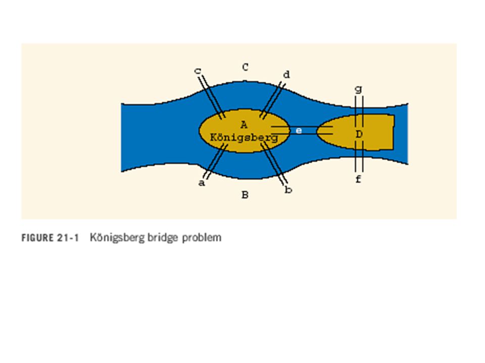
4. Introduction This chapter explores graphs and their applications in computer science In 1736, the following problem was posed: In the town of Königsberg, the river Pregel flows around the island Kneiphof and then divides into two The river has four land areas (A, B, C, D) −The land areas are connected using seven bridges, labeled a, b, c, d, e, f, and g

6. Introduction (continued) Starting at one land area, is it possible to walk across all the bridges exactly once and return to the starting land area? In 1736, Euler represented the bridge problem as a graph and answered the question in the negative.

7. Introduction (continued) Over the past 200 years, graph theory has been applied to a variety of problems Graphs are used to model electrical circuits, chemical compounds, highway maps, etc. Graphs are used in the analysis of electrical circuits, finding the shortest route, project planning, linguistics, genetics, social science

8. Let X be a set. If a is an element of X, then we write a  X. (The symbol “  ” means “belongs to.”) A set Y is called a subset of X if every element of Y is also an element of X. If Y is a subset of X, we write Y  X. (The symbol “  ” means “is a subset of.”) The intersection of sets A and B, written A  B, is the set of all the elements that are in A and B; that is, A  B =  x | x  A and x  B . (The symbol “  ” means “intersection.”)

9. The union of sets A and B, written A  B, is the set of all the elements that are in A or in B; that is, A  B =  x | x  A or x  B . The symbol “  ” means “union.” Note that x  A  B means x is in A or x is in B or x is in both A and B. Also, the symbol “  ” is read as “such that.” For sets A and B, the set A  B is the set of all the ordered pairs of elements of A and B; that is, A  B =  (a, b) | a  A, b  B .

10. A graph G is a pair, G = (V, E), where V is a finite nonempty set, called the set of vertices of G, and E  V  V. E is called the set of edges. Let V(G) denote the set of vertices and E(G) denote the set of edges of a graph G. If the elements of E(G) are ordered pairs, G is called a directed graph or digraph; otherwise, G is called an undirected graph. In an undirected graph, the pairs (u, v) and (v, u) represent the same edge. If (u, v) is an edge in a directed graph, then sometimes the vertex u is called the origin of the edge, and the vertex v is called the destination. Let G be a graph. A graph H is called a subgraph of G if V(H)  V(G) and E(H)  E(G); that is, every vertex of H is a vertex of G, and every edge in H is an edge in G.

11. A graph can be shown pictorially. The vertices are drawn as circles, and a label inside the circle represents the vertex. In an undirected graph, the edges are drawn using lines. In a directed graph, the edges are drawn using arrows. In a directed graph the tail of a pictorial directed edge is the origin, and the head is the destination.

14. For the graphs of Figure 21-4, we have V(G 1 ) = {1, 2, 3, 4, 5} E(G 1 ) = {(1, 2), (1, 4), (2, 5), (3, 1), (3, 4), (4, 5)} V(G 2 ) = {0, 1, 2, 3, 4,} E(G 2 ) = {(0, 1), (0, 3), (1, 2), (1, 4), (2, 1), (2, 4), (4, 3)} V(G 3 ) = {0, 1, 2, 3, 4, 5, 6, 7, 8, 9, 10} E(G 3 ) = {(0, 1), (0, 5), (1, 2), (1, 3), (1, 5), (2, 4), (4, 3), (5, 6), (6, 8), (7, 3), (7, 8), (8, 10), (9, 4), (9, 7), (9, 10)}

15. Let G be an undirected graph. Let u and v be two vertices in G. Then u and v are called adjacent if there is an edge from one to the other; that is, (u, v)  E(G). Let e = (u, v) be an edge in G. We then say that edge e is incident on the vertices u and v. An edge incident on a single vertex is called a loop. If two edges, e 1 and e 2, are associated with the same pair of vertices, then e 1 and e 2 are called parallel edges. A graph is called a simple graph if it has no loops and no parallel edges. There is a path from u to v if there is a sequence of vertices u 1, u 2,..., u n such that u = u 1, u n = v, and (u i, u i + 1 ) is an edge for all i = 1, 2,..., n − 1. Vertices u and v are called connected if there is a path from u to v. A simple path is a path in which all the vertices, except possibly the first and last vertices, are distinct. A cycle in G is a simple path in which the first and last vertices are the same.

16. G is called connected if there is a path from any vertex to any other vertex. A maximal subset of connected vertices is called a component of G. Let G be a directed graph, and let u and v be two vertices in G. If there is an edge from u to v, that is, (u, v)  E(G), then we say that u is adjacent to v and v is adjacent from u. The definitions of the paths and cycles in G are similar to those for undirected graphs. G is called strongly connected if any two vertices in G are connected. Consider the directed graphs of Figure 21-4. In G 1, 1-4-5 is a path from vertex 1 to vertex 5. There are no cycles in G 1. In G 2, 1-2-1 is a cycle. In G 3, 0-1-2-4-3 is a path from vertex 0 to vertex 3; 1-5-6-8- 10 is a path from vertex 1 to vertex 10. There are no cycles in G 3.

17. To write programs that process and manipulate graphs, the graphs must be stored in computer memory A graph can be represented in several ways: −Adjacency matrices −Adjacency lists

18. Let G be a graph with n vertices, where n  0. Let V(G) =  v 1, v 2,..., v n . The adjacency matrix A G of G is a two-dimensional n  n matrix such that the (i, j)th entry of A G is 1 if there is an edge from v i to v j ; otherwise, the (i, j)th entry is zero. That is, In an undirected graph, if (v i, v j )  E(G), then (v j, v i )  E(G), so A G (i, j) = 1 = A G (j, i). The adjacency matrix of an undirected graph is symmetric.

19. Consider the directed graphs of Figure 21-4.

21. Let G be a graph with n vertices, where n > 0 Let V(G) = {v 1,v 2,…,v n } In the adjacency list representation, corresponding to each vertex, v, there is a linked list where each node of the linked list contains the vertex, u, such that (u,v)  E(G)

22. Adjacency Lists (continued) With n nodes, we use an array, A, of size n, such that A[i] is a pointer to the linked list containing the vertices to which v i is adjacent Each node has two components, say vertex and link −The component vertex contains the index of the vertex adjacent to vertex i

25. Operations commonly performed on a graph: −Create the graph −Clear the graph which makes the graph empty −Determine whether the graph is empty −Traverse the graph −Print the graph The adjacency list (linked list) representation: −For each vertex, v, the vertices adjacent to v are stored in the linked list associated with v −To manage the data in a linked list, we use the class unorderedLinkedList, discussed in Chapter 17

29. Traversing a graph is similar to traversing a binary tree, except that −A graph might have cycles −Might not be able to traverse the entire graph from a single vertex The two most common graph traversal algorithms: −Depth first traversal −Breadth first traversal

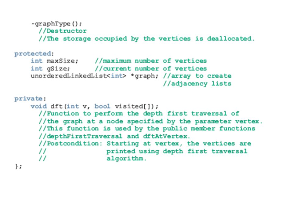
30. Depth First Traversal Depth first traversal at a given node, v: 1.Mark node v as visited 2.Visit the node 3.For each vertex u adjacent to v if u is not visited Start the depth first traversal at u

31. A depth first ordering of the vertices of the graph G3 in Figure 21-7 is: 0 1 2 4 3 5 6 8 10 7 9

32. The general algorithm to do a depth first traversal at a given node, v, is 1.Mark node v as visited 2.Visit the node 3.For each vertex u adjacent to v if u is not visited start the depth first traversal at u

34. In the preceding code, note that the statement linkedListIterator graphIt; declares graphIt to be an iterator. In the for loop, we use it to traverse a linked list (adjacency list) to which the pointer graph[v] points. The statement int w = *graphIt; The expression *graphIt returns the label of the vertex, adjacent to the vertex v, to which graphIt points.

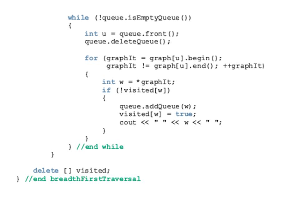
37. Breadth first traversal of a graph is similar to traversing a binary tree level by level Starting at the first vertex, the graph is traversed as much as possible −Then go to the next vertex that has not yet been visited Use a queue to implement the breadth first search algorithm

38. A breadth first ordering of the vertices of the graph G 3 in Figure 21-7 is: 0 1 5 2 3 6 4 8 10 7 9

39. The general algorithm is:

42. Shortest Path Algorithm The edges connecting two vertices can be assigned a non-negative real number called the weight of the edge In a weighted graph, every edge has a non- negative weight The weight of the path P is the sum of the weights of all edges on the path P, which is also called the weight of v from u via P

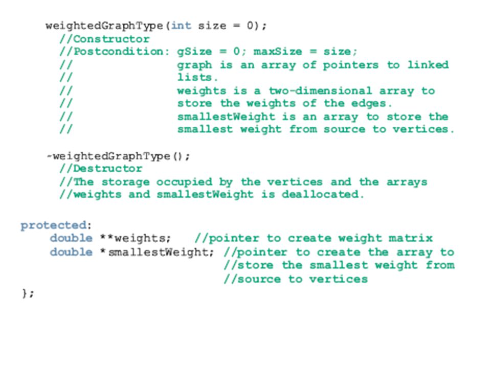
43. Shortest Path Algorithm (continued) The shortest path is the path with the smallest weight The shortest path algorithm, called the greedy algorithm, was developed by Dijkstra Let G be a graph with n vertices, where n ≥ 0 Let V(G) = {v 1, v 2,..., v n }, and W be a two- dimensional n × n matrix

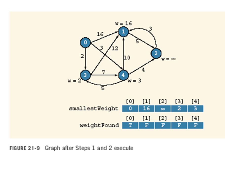
46. Shortest Path Algorithm (continued) Shortest path algorithm: 1.Initialize the array smallestWeight so that smallestWeight[u] = weights[vertex,u]. 2.Set smallestWeight[vertex] = 0 3.Find the vertex, v, which is closest to vertex for which the shortest path has not been determined

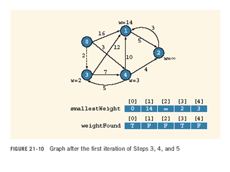
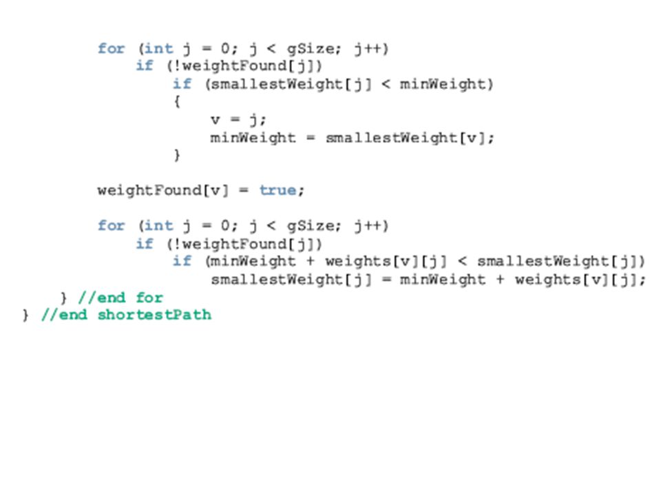
47. Shortest Path (continued) 4.Mark v as the (next) vertex for which the smallest weight is found 5.For each vertex w in G, such that the shortest path from vertex to w has not been determined and an edge (v, w) exists: If the weight of the path to w via v is smaller than its current weight, update the weight of w to the weight of v + the weight of the edge (v, w)

58. Due to financial hardship, the company needs to shut down the maximum number of connections and still be able to fly from one city to another (the flights need not be direct). The graphs of Figure 21-15(a), (b), and (c) shows three different solutions.

60. A (free) tree T is a simple graph such that if u and v are two vertices in T, then there is a unique path from u to v. A tree in which a particular vertex is designated as a root is called a rooted tree. If a weight is assigned to the edges in T, T is called a weighted tree. If T is a weighted tree, the weight of T, denoted by W(T), is the sum of the weights of all the edges in T. A tree T is called a spanning tree of graph G if T is a subgraph of G such that V(T) = V(G), that is, all the vertices of G are in T. Suppose G denotes the graph of Figure 21-14. Then the graphs of Figure 21-15 show three spanning trees of G.

61. Theorem: A graph G has a spanning tree if and only if G is connected. In order to determine a spanning tree of a graph, the graph must be connected. Let G be a weighted graph. A minimal spanning tree of G is a spanning tree with the minimum weight.

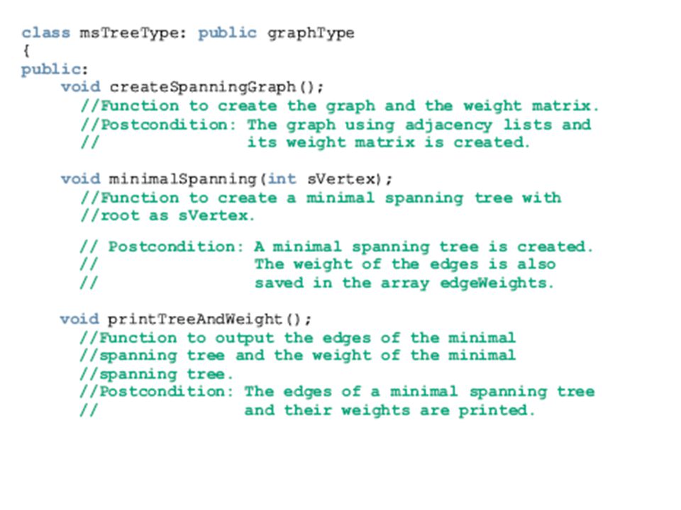
62. Minimal Spanning Tree (continued) There are two well-known algorithms to find a minimal spanning tree of a graph: −Prim’s algorithm −Kruskal’s algorithm

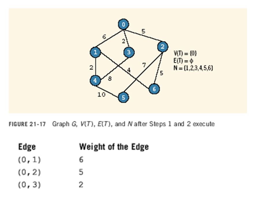
63. Prim’s algorithm builds the tree iteratively by adding edges until a minimal spanning tree is obtained. We start with a designated vertex, which we call the source vertex. At each iteration, a new edge that does not complete a cycle is added to the tree.

64. The general form of Prim’s algorithm is

79. Summary A graph G is a pair, G = (V, E) In an undirected graph G = (V, E), the elements of E are unordered pairs In a directed graph G = (V, E), the elements of E are ordered pairs A graph H is a subgraph of G if every vertex of H is a vertex of G and every edge in H is an edge in G Two vertices in an undirected graph are adjacent if there is an edge between them

80. Summary (continued) Loop: An edge incident on a single vertex Simple graph: no loops and no parallel edges Simple path: all the vertices, except possibly the first and last vertices, are distinct Cycle: a simple path in which the first and last vertices are the same Undirected graph is called connected if there is a path from any vertex to any other vertex

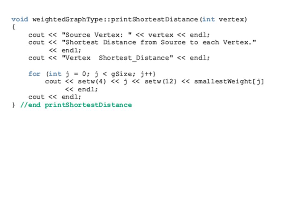
81. Summary (continued) Shortest path algorithm gives the shortest distance for a given node to every other node in the graph In a weighted graph, every edge has a non- negative weight A tree in which a particular vertex is designated as a root is called a rooted tree A tree T is called a spanning tree of graph G if T is a subgraph of G such that V(T) = V(G) (all vertices of G are in T)