1. Statistical Techniques I
EXST7005
The F distribution

2. The F test This test can be used to either,
test the equality of population variances - our present topic
test the equality of population means (this will be discussed later under ANOVA)
The F test is the ratio of two variances (the ratio of two chi square distributions)
Given two populations
Population 1 Population 2
Mean m m2
Variance s s2

3. The F test (continued) Two populations
Draw a sample from each population
Population 1 Population 2
Sample size n n2
d.f g g2
Sample mean `Y `Y2
Sample variance S S2

4. The F test (continued) To test the Hypothesis H0: s12 = s22
H1: s12 ¹ s22 (one sided also possible)
use F = s12 / s22
which has an expected value of 1 under the null hypothesis, but in practice there will be some variability so we need to define some reasonable limits and this will require another statistical distribution.

5. The F distribution
1) The F distribution is another family of distributions, each specified by a PAIR of degrees of freedom, g1 and g2.
g1 is the d. f. for the numerator
g1 is the d. f. for the denominator
Note: the two samples do not have to be of the same size and usually are not of the same size.
2) The F distribution is an asymmetrical distribution with values ranging from 0 to ¥, so [0 £ F £ ¥].

6. The F distribution (continued)
3) There is a different F distribution for every possible pair of degrees of freedom.
4) In general, an F value with g1 and g2 d.f. is not the same as an F value with g2 and g1 d.f., so order is important.
i.e. Fg1,g2 ¹ Fg2,g1 usually
5) The expected value of any F distribution is 1 if the null hypothesis is true.

7. The F distribution F distribution with 1, 5 d.f.
0.00
0.50
1.00
1.50
2.00
2.50
3.00
3.50
4.00

8. The F tables
1) The numerator d.f. (g1) are given along the top of the page, and the denominator d.f. (g2) are given along the left side of the page.
Some tables give only one F value at each intersection of g1 and g2. The whole page would be for a single a value and usually several pages would be given.

9. The F tables (continued)
Our tables will give four values at the intersection of each g1 and g2, each for a different a value. These a values are given in the second column from the left.
Our tables will have two pages.
Only a very few probabilities will be available, usually 0.05, 0.025, 0.01 and 0.005, and sometimes
Only the upper tail of the distribution is given.

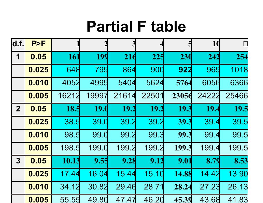
10. Partial F table d.f. P>F 1 2 3 4 5 10 ¥ 1 0.05 161 199 216 225 230
242
254
0.025
648
799
864
900
922
969
1018
0.010
4052
4999
5404
5624
5764
6056
6366
0.005
16212
19997
21614
22501
23056
24222
25466 2
0.05
18.5
19.0
19.2
19.2
19.3
19.4
19.5
0.025
38.5
39.0
39.2
39.2
39.3
39.4
39.5
0.010
98.5
99.0
99.2
99.3
99.3
99.4
99.5
0.005
198.5
199.0
199.2
199.2
199.3
199.4
199.5 3
0.05
10.13
9.55
9.28
9.12
9.01
8.79
8.53
0.025
17.44
16.04
15.44
15.10
14.88
14.42
13.90
0.010
34.12
30.82
29.46
28.71
28.24
27.23
26.13
0.005
55.55
49.80
47.47
46.20
45.39
43.68
41.83

11. Working with F tables
The F tables are used in a fashion similar to other statistical tables.
For the two degrees of freedom (be sure to keep numerator and denominator degrees of freedom distinct).
For a selected probability value
Find the corresponding F value.

12. Using the F tables EXAMPLE of F table use, one tailed example:
Find F with (5,10) d.f. for a = 0.05
find F0.05 such that P[F ³ F0.05, 5, 10 d.f. ] = 0.050
where g1 = 5 and g2 = 10

13. Using the F tables (continued)
For F5, 10 d.f. The tabular values are listed as 3.33, , ,
These represent
P[F5, 10 d.f. ³ 2.52] = (Not in your table)
P[F5, 10 d.f. ³ 3.33] =
P[F5, 10 d.f. ³ 4.24] =
P[F5, 10 d.f. ³ 5.64] =
P[F5, 10 d.f. ³ 6.87] =

14. Using the F tables (continued)
so the value we are looking for is 3.33, for this value P[F5, 10 d.f. ³ 3.33] = 0.050
note that since this is a 1 tailed value, then
P[F5, 10 d.f. £ 3.33] = 0.950
so the two sides sum to 1
Also note that if we reverse the d.f., we find that P[F10, 5 d.f. ³ 4.74] = , so the F values generally differ when d.f. are reversed

15. More working with F tables
Only the upper tail of the distribution is given. There are three reasons for this.
The F tests in Analysis of Variance (ANOVA) are usually one tailed tests, where the lower tail is not needed.
The need to calculate the lower tail can be eliminated in some two-tailed cases.
The value of F for the lower tail can be found by transformation of values from the upper tail.

16. Calculating lower tail values for the F distribution
It is possible to calculate the value of the lower tail from the tables providing the values for the upper tail.
To obtain the lower tail for a value Fg1,g2 for a particular value of a
First obtain the value in the upper tail for Fg2,g1 for the same value of a (note the change in order of the d.f.)
Then calculate 1/Fg2,g1 to get the lower tail.

17. F table : two-tailed example
Find F with (8,10) d.f. for a = 0.05
find Fa = 0.05/2, 8, 10 lower and Fa = 0.05/2, 8, 10 such that
P[Fa = 0.975, 8, 10 £ F £ Fa = 0.025, 8, 10]=0.950
where g1 = 8 and g2 = 10

18. F table : two-tailed example (continued)
For the upper tail, the value we are looking for is 3.85, for this value
P[F8, 10 ³ 3.85] = 0.025
note that we use only a/2 as the probability for one of the two tails

19. F table : two-tailed example (continued)
in order to find the lower tail, we reverse the d.f., we find that
P[F10, 8 ³ 4.30] = and then calculate
F8, 10 d.f. lower limit = 1/F10,8 = 1/4.30 =
note the reversal of the order of the degrees of freedom

20. Numerical example of an F-test of hypothesis
The concentration of blue green algae was obtained for 7 phytoplankton-density samples taken from each of two lake habitats. Determine if there is a difference in the variability of phytoplankton density between the two habitats.
1) H0: s12 = s22
2) H0: s12 ¹ s22

21. Numerical example of an F-test of hypothesis (continued)
3) Assume: Independence (randomly selected samples) and that BOTH populations are normal
4) a = 0.05
5) Draw a sample of 7 from each habitat, calculate the variances and the F ratio.

22. Numerical example of an F-test of hypothesis (continued)
Habitat 1
Habitat 2
Observation 1
7.6
5.9
Observation 2
0.4
3.8
Observation 3
1.1
6.5
Observation 4
3.2
18.3
Observation 5
6.5
18.2
Observation 6
4.1
16.1
Observation 7
4.7
7.6

23. Numerical example of an F-test of hypothesis (continued)
Statistic
Habitat 1
Habitat 2
SYi
27.6
76.4
SYi2
150.52
1074.6 CF
41.70
240.75 g 6 6 S2
6.95
40.12 S
2.64
6.33
Mean (`Y)
3.94
10.91

24. Numerical example of an F-test of hypothesis (continued)
Then calculate the F value as;
F = S12 / S22 = 6.95 / =
6) Calculate the critical region, given a=0.05 and a TWO TAILED alternative, and knowing that the degrees of freedom are g1=6 and g2=6, (note that both are equal).

25. Numerical example of an F-test of hypothesis (continued)
Calculate
P[Flower £ F £ Fupper] = P[Flower £ F] + P[F ³ Fupper] =
P[F ³ Fupper] = we can get directly from the table, Fa=0.05, 6, 6 = 5.82
P[Flower £ F] = we calculate as
1/P[F ³ Fupper] = 1/ =
This case is uncommon because d.f. upper = d.f. lower, so the F values are the same.

26. Numerical example of an F-test of hypothesis (continued)
6 continued) From the critical limits we can state that
P[Flower £ F £ Fupper] =
P[ £ F £ 5.82] = 0.05
and since our calculated F value is between these values (F = ) we would fail to reject the Null Hypothesis, concluding that the data is consistent with the Null Hypothesis. (But it was close.)

27. Some notes on F tests
NOTE that in this case the smaller value fell in the numerator. As a result, we were comparing the F value to the lower limit.
However, FOR TWO TAILED TESTS, IT MAKES NO DIFFERENCE WHICH FALLS IN THE NUMERATOR, AND WHICH IN THE DENOMINATOR. As a result, we can ARBITRARILY place the LARGER value in the numerator, and COMPARE THE F value to the UPPER LIMIT.

28. Some notes on F tests (continued)
This saves calculating the lower limit.
i.e. Calculate F = S2larger /S2smaller
BUT, don't forget that this arbitrary placing of the larger variance estimate in the NUMERATOR is done for TWO SAMPLE TESTS ONLY, and that therefore we want to test against Fa/2.

29. Some notes on F tests (continued)
Three common cases in F testing (actually two common and one not so common).
1) Frequently, particularly in ANOVA (to be covered later), we will test H0: s12 = s22 against the alternative, H1: s12 s22.
then we ALWAYS form the F value as F = S12 / S22. We put the one we EXPECT to be larger in the numerator for a one tailed test!
If F < 1 we don't even need to look up a value in the table, it cannot be "significant".

30. Some notes on F tests (continued)
2) Normal 2 tailed tests (common in 2 sample t-tests to be covered later) will test H0:s12=s22 against the alternative, H1:s12¹s22.
then we can form the F value as F=S2larger/S2smaller.
This is a 2-tailed test and it is tested against the upper tail with a/2 in the upper tail.
There is no way that we can get a calculated F < 1.

31. Some notes on F tests (continued)
3) If both the upper and lower bounds are required (not common, found mostly on EXAMS in basic statistics) then we will be testing H0:s12=s22 against the alternative H1:s12¹s22.
We can form the F value any way we want, with either the larger or smaller variance in the numerator.
This is a 2 tailed test with a/2 in each tail, and F can be any value (0 to ¥)

32. Summary
The F distribution is ratio of two variances (i.e. two Chi square distributions) and is used test used to test two variances for equality. H0: s12 = s22
The distribution is an asymmetrical distribution with values ranging from 0 to ¥, and an expected value of 1.
The F tables require two d.f. (numerator and denominator) and give only a very few critical values.

33. Summary (continued)
Many, perhaps most, F tests will be directional. For the tests the variance that is EXPECTED to be larger goes in the numerator whether it is larger or not and we test against the upper tail with a probability equal to a.
For the non-directional alternative we may arbitrarily place the larger variance in the numerator and test against the upper tail, but don't forget to test against a/2.