1. We start Part II (Quantifying Uncertainty) today Lab 2 - Equations Tomorrow - Tue 3-5 or 7-9 PM - SN 4117 Assignment 2 – Data Equations Due Wednesday

2. Data = Model + Residual Chapter 5 Data Equations Data = Model + Residual

3. Data Equations Central concept in the course We’ll teach a general approach that will allow you to set up an appropriate analysis of data You don’t have to worry about whether you have selected the ‘right’ test We are going to use data equations to compare models to data Data = Model + Residual

4. Flexible approach Data = Model + Residual

5. Symbolic expression  Analyse data Increase confidence using model triangle – Link symbols with graphical and verbal model Data Verbal GraphicalFormal

6. Assessing fit We’ll use data equations to measure: – How well the model fits the data (goodness of fit) – Error rate Model Plant height Time in sunlight Data We do not expect a perfect fit But model and observed values should be close

7. Definition Three terms: Y=Ŷ+εY=Ŷ+ε DataModelResidual ObservedExpectedError Fitted Residuals: ε= Y -Ŷ

8. e.g. Dobzhansky’s Fruit Flies Dobzhansky pioneered work on fruit fly evolutionary genetics in the lab and field One research question he addressed was: – Does genetic variability decrease at higher altitude, due to stronger selection in extreme environments? Nothing in Biology Makes Sense Except in the Light of Evolution

9. e.g. Dobzhansky’s Fruit Flies Nothing in Biology Makes Sense Except in the Light of Evolution Heterozygosity H (%) Elevation E (km) 0.590.26 0.370.91 0.411.4 0.41.89 0.312.44 0.182.62 0.23.05 Nothing in Biology Makes Sense Except in the Light of Statistics ?

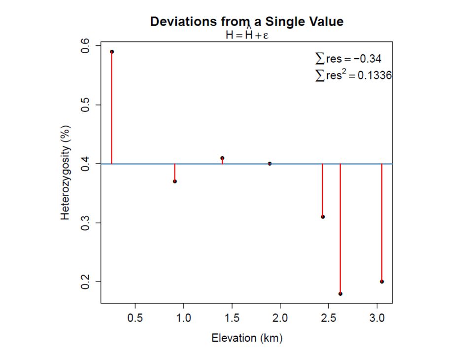
10. Heterozygosity H (%) Elevation E (km) 0.590.26 0.370.91 0.411.4 0.41.89 0.312.44 0.182.62 0.23.05 Model? Heterozygosity in Drosophila = 40% Data = Model + Residual H =Ĥ + ε H = 40% + ε Many options First we’ll check deviance from a single value

11. ==== ++++ 0.59=0.4+0.190.0361 0.37=0.4+-0.030.0009 0.41=0.4+0.010.0001 0.4= +0.000.0000 0.31=0.4+-0.090.0081 0.18=0.4+-0.220.0484 0.2=0.4+-0.200.0400 ∑-0.340.1336 With this simple model, we can form 7 data equations Summed residuals is a measure of bias Summed residuals 2 is a measure of goodness of fit

13. What if the parameter is unknown?

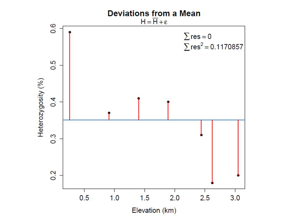
14. ==== ++++ 0.59=0.3514+0.23860.0569 0.37=0.3514+0.01860.0003 0.41=0.3514+0.05860.0034 0.4=0.3514+0.04860.0024 0.31=0.3514+-0.04140.0017 0.18=0.3514+-0.17140.0294 0.2=0.3514+-0.15140.0229 ∑00.1171 Form 7 data equations

17. Single value vs. Mean model Mean model: unbiased and better fit But biological criteria have been replaced by statistical criteria

18. e.g. Dobzhansky’s Fruit Flies Nothing in Biology Makes Sense Except in the Light of Evolution Heterozygosity H (%) Elevation E (km) 0.590.26 0.370.91 0.411.4 0.41.89 0.312.44 0.182.62 0.23.05 What about elevation?...don't you remember my question? Does genetic variability decrease at higher altitude, due to stronger selection in extreme environments?

19. %/kmkm%%

20. Heterozygosity H (%) Elevation E (km) 0.59 0.26 0.2 3.05

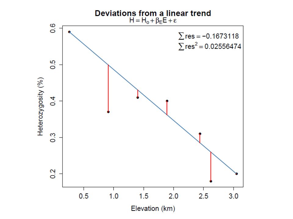
22. ==== ++++ 0.260.59=0.5900+0.0000 0.910.37=0.4991+-0.12910.0167 1.40.41=0.4306+-0.02060.0004 1.890.4=0.3622+0.03780.0014 2.440.31=0.2853+0.02470.0006 2.620.18=0.2601+-0.08010.0064 3.050.2=0.2000+0.0000 ∑-0.17000.0253 With this equation, we can calculate fitted values ? ? ? ? ? ? ? ? ? ? ? ? ? ?

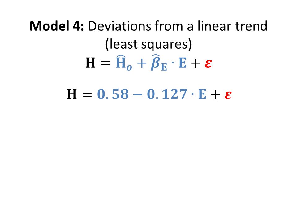
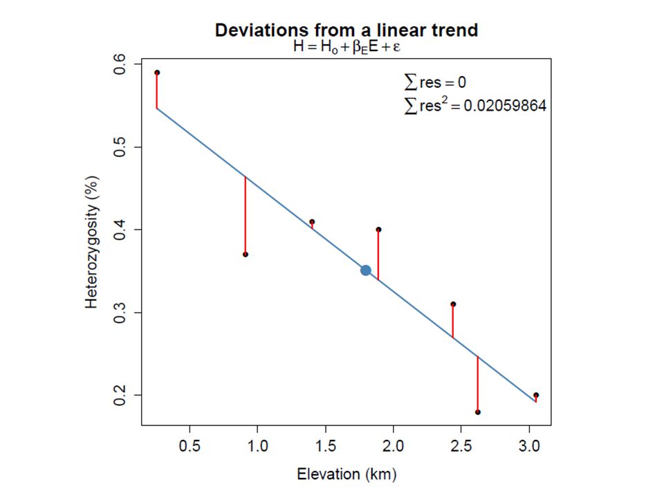
24. There’s a better way to estimate slope

28. Model comparison ∑ res = -0.34 ∑ res = 0 ∑ res = -0.17 ∑ res = 0 Two unbiased models ∑ res 2 = 0.1171 ∑ res 2 = 0.0204 Reduction in squared deviance ∑ res 2 = 0.0966