1. CE 3231 - Introduction to Environmental Engineering and Science Readings for This Class: 5.5-5.6 O hio N orthern U niversity Introduction Chemistry, Microbiology & Material Balance Water & Air Pollution Env Risk Management Atmospheric Dispersion (Modeling) The atmosphere is a complex and dynamic system. Under certain conditions, the atmosphere can trap pollution at the Earth surface and lead to adverse health effects. Understanding near surface atmospheric conditions and their effect on pollution dispersion is the point of this lecture.

2. Lecture 27 Atmospheric Dispersion (Modeling) (Air Quality II)

3. Introduction to Air Quality

4. Air Quality II  Topics Covered Include:  Adiabatic Lapse Rate  Atmospheric Stability  Inversions  Plume Shapes and Dynamics  Gaussian Plume Modeling  Simplified Model to Predict Downwind Ground Level Pollution

5. Adiabatic Lapse Rate Temperature drops as you increase in altitude Γ dry = 9.76 or 5.4 Γ saturated = 6in tropopause

6. Atmospheric Stability Stable Air – Air mass remains at set altitude – Problematic for pollution Unstable Air – Air mass changes altitude – Favors mixing and pollution dispersion

7. Temperature Inversions – Stable atmosphere – Nocturnal cooling – Earth cools rapidly, traps colder air on bottom – Pollution can get trapped near surface – Daytime sunlight radiates ground and breaks inversion http://www.metoffice.gov.uk/education/secondary/students/smog.html

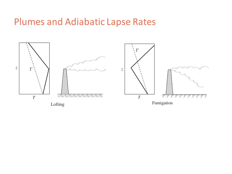
8. Plumes and Adiabatic Lapse Rates

11. Gaussian Plume Modeling

13. where: C (x,y) = downwind conc. at ground level(z=0), g/m 3 Q = emission rate of pollutants, g/s  y,  z = plume standard deviation, m u H = wind speed, m/s x,y, and z = distance, m H = stack height

14. How will the model change for ground-level along the plume?

15. Simplified Plume Modeling (Downwind Ground-Level Concentration)

16. Gaussian Plume Modeling where: C (x,0) = downwind conc. at ground level (z=0, y=0), g/m 3 Q = emission rate of pollutants, g/s  y,  z = plume standard deviation, m u H = wind speed, m/s x,y, z and H = distance, m

17. Dispersion Constants A – very unstable; B – moderately unstable; C- slightly unstable, D – neutral, E – slightly stable; F – stable

18. Gaussian Plume Modeling A new power plant releases SO 2 at a legally allowable rate of 6.5x10 8  g SO 2 /sec. The stack has an effective height of 300 m. An anemometer on a 10 m pole measures 2.5 m/s of wind, and it is a cloudy summer day. Predict the ground- level concentration of SO 2 4 km directly downwind.

19. Gaussian Plume Modeling Q = 6.5x10 8  g SO 2 /sec H = 300 m. U = 2.5 m/s @ 10 m X= 4 km Atmospheric condition = ? u H = ?  y,  z = ?

20. Finding the Atmospheric Condition Atmospheric Condition A – very unstable, sunny day with wind speed < 3 m/s B – moderately unstable, sunny day clear night with winds between 3 – 5 m/s C- slightly unstable, sunny day with winds > 5 m/s D – neutral cloudy or overcast day; cloudy night winds > 3 m/s; clear night winds > 5 m/s E – slightly stable cloudy or overcast night winds < 3 m/s F – stable clear night winds < 5 m/s

21. Finding u H Atmospheric Condition (p value) A – (0.15) B – (0.15) C- (0.2) D – (0.25) E – (0.4) F – (0.6)

22. Finding  y,  z D – neutral @ 4 km  y = 250 m and  z = 80 m

23. Gaussian Plume Modeling Q = 6.5x10 8  g SO 2 /sec H = 300 m. U = 2.5 m/s @ 10 m X= 4 km Atmospheric condition = D u H = 5.85 m/s  y = 250 m  z = 80 m

24. Gaussian Plume Modeling A new power plant releases SO 2 at a legally allowable rate of 6.5x10 8  g SO 2 /sec. The stack has an effective height of 300 m. An anemometer on a 10-mile pole measures 2.5 m/s of wind, and it is a cloudy summer day. Predict the ground-level concentration of SO 2 4 km directly downwind.