1. Draft Status of the U.S. petrale sole resource in 2012 STAR Panel Melissa Haltuch 1, Kotaro Ono 2, Juan Valero 3 1 NWFSC, Seattle 2 UW, SAFS, Seattle 3 CAPAM, La Jolla 13 May 2013

2. Outline Introduction Introduction Data Data –Fishery Independent –Biological –Fishery Dependent Previous Modeling Previous Modeling Responses to 2011 STAR panel Responses to 2011 STAR panel General Model Description General Model Description Base Case Model Base Case Model –Sensitivity Analysis –Retrospective Analysis –Historical Assessment Analysis –Likelihood Profile –Harvest Projections

3. Introduction - Biology Right eyed flounder Right eyed flounder Gulf of Alaska to Baja California Gulf of Alaska to Baja California Soft bottoms Soft bottoms 550 m depth 550 m depth No genetic work No genetic work Adults migrate seasonally Adults migrate seasonally No strong indication of multiple stocks No strong indication of multiple stocks

4. Introduction - Fishery 1876 off of San Francisco, CA 1876 off of San Francisco, CA 1884-1885, established by 1937 in OR 1884-1885, established by 1937 in OR Began about 1932, established by 1936 in WA Began about 1932, established by 1936 in WA Early concerns about stock depletion in the 1950s Early concerns about stock depletion in the 1950s Targeting of winter spawning aggregations developed through the 1950s and 1960s Targeting of winter spawning aggregations developed through the 1950s and 1960s By 1980s winter catches exceeded summer catches in many years By 1980s winter catches exceeded summer catches in many years

5. Introduction - Management AssessmentStatusYear(s)OFLACL 1984-1999 Near Target 1983-20063200-27623200-2762 2005Precautionary2007-20093025-28112499-2433 2009-2011Overfished2010-20122751-12791200-1160 Management actions since the late 1990s Management actions since the late 1990s –Area closures –Trip limits –Gear modifications –IFQ

6. Triennial survey 1977 (excluded) 1977 (excluded) –Depth: 91-457 meters 1980-1992 1980-1992 –Depth: 55-366 meters 1995-2004 1995-2004 –Depth: 55-500 meters Run by RACE until 2004 when run by FRAM Run by RACE until 2004 when run by FRAM Random trawls on systematic line transects Random trawls on systematic line transects

7. Triennial Survey Timing

8. NWFSC survey 1999-2002 1999-2002 –surveyed 183-1280 meters –Did not always go as far south 2003 through 2008 2003 through 2008 –55-1280 meters –32.5° to 48.17° Random trawl locations Random trawl locations Random vessels chosen each year Random vessels chosen each year

9. Survey differences TriennialNWFSC Systematic random stations on equally spaced transects Randomly selected within stratified random block AK class commercial trawlers 65-147 feet WC commercial trawlers 65-92 feet High opening NorEastern trawl 4 panel Aberdeen style trawl 250 feet net to doors 205 feet net to doors Roller gear (121 footrope) Continuous disk footrope (104) Bare wire bottom bridles 8 disks in wings 6 X 9 V-Door 5 X 7 V-Door 5 mesh, 3.5 codend, 1.25 liner 5.5 mesh, 5 cod end, 2 liner 30 minute tow 15 minute tow 3.0 knot towing speed 2.2 knot towing speed

10. Surveys Triennial Triennial –Two time series: 1980-1992 and 1995-2004 –Excluded the Conception area (S of 36°) –Biomass and length frequencies NWFSC NWFSC –One time series: 2003-2012 –All areas –Biomass, lengths, and age-at-length

11. Catch rates: Triennial

12. Catch rates: NWFSC

13. Density: NWFSC

14. Survey post-stratification Post-stratify depth using fish length Post-stratify depth using fish length –Ontogenetic movement to deeper water –Lai et al (2005) used Bayesian change-point analysis –Haltuch et al (2009) used a frequentist approach and came to same result –Significant split just greater than 100 m

15. Mean fish length vs depth

16. Survey stratification for GLMM/GLM Strata collapsed to satisfy condition of at least 3 positive observations in each year/area/depth stratum Strata collapsed to satisfy condition of at least 3 positive observations in each year/area/depth stratum Depths Depths –Triennial (Early and Late): 55-100 meters and 100+ m –NWFSC: 55-100 m, 100-183 m, 183+ m Areas Areas –Triennial Early Early –Shallow: Vancouver/Columbia, Eureka, Monterey/Conception –Deep: Vancouver/Columbia/Eureka, Monterey/Conception Late: Late: –Shallow: Vancouver/Columbia, Eureka, Monterey/Conception –Deep: Vancouver/Columbia, Eureka, Monterey, Conception –NWFSC Shallow/Middle – Vancouver/Columbia, Eureka, Monterey, Conception Shallow/Middle – Vancouver/Columbia, Eureka, Monterey, Conception Deep – Combined Eureka-Columbia/Vancouver Deep – Combined Eureka-Columbia/Vancouver

17. Model based biomass estimates Delta-GLMM Delta-GLMM –NWFSC: random year:vessel effects –Triennial: NO random vessel effects –Fixed effects: year, strata, depth, year:strata Lognormal errors Lognormal errors MCMCs to determine variability MCMCs to determine variability

18. Model selection – residual deviance SurveyModelMean Tri_earlyGamma-Strata:YearFixed7814.3 Tri_earlyLognormal-Strata:YearFixed7655.1 Tri_lateGamma-Strata:YearFixed6903.1 Tri_lateLognormal-Strata:YearFixed6840.5 NWFSCGamma-Strata:YearFixed19885.2 NWFSCLognormal-Strata:YearFixed19723.7

19. Model fit - lognormal

20. Survey biomass estimates

21. Triennial length frequencies

22. NWFSC length frequencies

23. NWFSC age frequency

24. NWFSC survey length at age

25. Summary of survey data NWFSC survey has higher catch rates than the triennial survey, resulting in larger biomass estimates NWFSC survey has higher catch rates than the triennial survey, resulting in larger biomass estimates 2004 triennial survey catch rates are on average higher than rest of triennial series 2004 triennial survey catch rates are on average higher than rest of triennial series Trend in NWFSC survey peaks in 2004, declines through 2008, and increases after 2009 Trend in NWFSC survey peaks in 2004, declines through 2008, and increases after 2009 –Smaller and younger fish observed in 2008-2010

26. Biological Data - Weight-Length NWFSC Survey NWFSC Survey

27. Biological Data – Maturity at length Oregon Oregon Washington Washington 2002 2002

28. Biological Data – Natural Mortality 1940s Catch Curve 1940s Catch Curve –M: 0.18-0.26 –F: 0.19-0.21 Hoenigs Method Hoenigs Method –0.15 max age of 30 (female petrale sole live at least 30 years) (female petrale sole live at least 30 years) Hamel prior Hamel prior –M median: 0.206, SD: 0.16 –F median: 0.151, SD: 0.206

29. Ageing Precision and Bias 3 Labs 3 Labs –Cooperative Ageing Lab OR and CA commercial (1986-present), NWFSC Survey OR and CA commercial (1986-present), NWFSC Survey –WDFW –CDFG (only samples pre ~1980s) Surface ages Surface ages –pre 1980s –OR 2001-2004 Combo method Combo method –OR 1981-1984, 1987-1988, 1991-1997 (reader issues) –WA ~1990 – 2009 Break and Burn Break and Burn –NWFSC survey –OR (1985-1986, 1989-1990, 1998-1999, 2007-present) –WA (2009-present) –CA (1986-present)

30. Ageing Error Methods Punt et al. 2008; simulation tested Punt et al. 2008; simulation tested Estimate ageing error assuming one reader is unbiased Estimate ageing error assuming one reader is unbiased –based on bomb radiocarbon age validation Data pooled across reader Data pooled across reader Early surface age error estimate for pre-1990s samples Early surface age error estimate for pre-1990s samples Sample sizes – 100s of double and triple reads Sample sizes – 100s of double and triple reads Model selection – AIC Model selection – AIC –Shape of bias, shape of error, minus age, and plus age

31. Ageing Error - Results

32. Pikitch Discard Data

33. WCGOP Observer Lengths SummerWinter

34. WCGOP Observer Data 2002-2010– Summer Spatial distribution of observed catch

35. WCGOP Observer Data 2002-2010 – Winter Spatial distribution of observed catch

36. Fraction Discarded Discard/Total Catch FishingNorth winterNorth summerSouth winterSouth summer YearMeanSDMeanSDMeanSDMeanSD 19850.02220.11030.03460.0419 19860.02150.11620.03430.0432 19870.0270.11860.03150.045 20020.00770.00340.18560.02530.03720.02440.05690.0158 20030.010.00640.11110.02520.00620.00260.03250.0126 20040.00190.00080.08430.02440.05260.05210.03430.0153 20050.00130.00090.04210.01120.00690.00710.01220.0035 20060.01310.00730.0780.01710.05980.04460.0360.0157 20070.00370.00150.11380.02320.01940.01390.0610.0209 20080.02750.01460.05020.01670.00990.00560.02590.0147 20090.02530.01510.20180.06730.02210.01470.02330.0082 20100.19710.04440.10370.03080.25840.07170.05540.0119 20110.001700.03700.000900.04110 20120.00060000.0046000

37. Commercial Length Comps – North Summer Winter

38. Commercial Age Comps Summer Winter

39. Landings

40. 2011 v. 2013 Landings

41. CPUE standardization steps: 1. Data filtering 2. Identify the covariates to use/test 3. Build a regression model that best fits the data 4. Create an index of abundance with some credibility interval

42. 1. Data Filtering Spatial Spatial Spatially defined fishing grounds 2003-2008 2003-2008 Summer – May-October Summer – May-October Shoreward of 75fm Shoreward of 75fm remove tows with flatfish catch rates in lower 10% remove tows with flatfish catch rates in lower 10% Winter – Nov-Feb Winter – Nov-Feb Seaward of 150fm Seaward of 150fm Remove tows with petrale catch rate in lower 10% Remove tows with petrale catch rate in lower 10% Data quality Remove Tows outside EEZ mid-water trawls Tow duration 0.2 hours Difference between map and logbook depths > 70 fm Tows 300 fm (S); 400 fm (W) Tow duration 4 hours (S); 6 hours (W) Vessels < 5 years in fishery (sensitivity test) Winter Nov-Dec data Output: average CPUE (lbs/hr) by fishing trip

43. 1. Data Filtering Tow by tow data Trip by trip data Summer North 7975218627 South 164056645 Winter North 109363984 South 28411307

44. 2. Covariates to test Models for each fleet separately: North winter, North summer, South winter, South summer Time: year, bimonth Space: spatial grid Vessel effects: port, vessel ID, gear, targeting

45. 2013 model stratification

46. 3. Model building Build a regression model - Data contains a lot of zero in addition to the positive data delta (hurdle) model - Mixed effect model with vessel as random effect Choose covariates through model selection (AIC) Check model assumptions

47. Changes from 2011 1. Summer data filtering corrected 2. Changed the reference level of the covariates during the index standardization to be the mean (continuous) or most frequently observed (categorical) index of abundance can be interpreted as index per reference unit calculate a confidence interval 3. Finer spatial stratification 4. Aggregate tow level data to trip level data Greater independence 5. fishing tactics covariates 6. Sensitivity to random vessel effects 7. WA and OR aggregated into North fleet

48. The 2011 best main effect models (determined after model selection) WinterSummer WA 43%30% OR 34%52% CA 40% Explained deviance

49. The 2011 best main effect models + removed tows outside EEZ WinterSummer WA 43%27% OR 34%42% CA 40% Explained deviance

50. The 2011 best main effect models + removed tows outside EEZ + change reference levels WinterSummer WA 43%27% OR 34%42% CA 40% Explained deviance

51. The 2011 best main effect models + removed tows outside EEZ + change reference levels + standardized the index by its geometric mean (change of scale) WinterSummer WA 43%27% OR 34%42% CA 40% Explained deviance

52. 2011 best main effect models + removed tows outside EEZ + change reference levels + standardized the index by its geometric mean (change of scale) 2011 best main effect models + trip level data WinterSummer WA 34%32% OR 35%47% CA 34%42% Explained deviance

53. 2011 best main effects models + trip level data 2013 best main effects models + trip level data WinterSummer WA 34%35% OR 34%48% CA 38%44% Explained deviance

54. 2013 best main effects models + trip level data The 2013 best main effects models + trip level data +targeting covariates WinterSummer WA 66% OR 74%71% CA 72%65% Explained deviance

55. The 2013 best main effects models + trip level data +targeting covariates The 2013 best main effects models + trip level data +targeting covariates + mixed effect model WinterSummer WA 44%67% OR 68%71% CA 74%65% Explained deviance

56. Model fits Lognormal component Summer OR Winter OR

57. Final index of abundance 2013 assessment has a different spatial set-up: North fishery ( WA+OR) and the South fishery (CA) Graphs are scaled so that the 2004 index = 1. WinterSummer North78%74% South74%65% Explained deviance

58. Final index of abundance with prediction interval

59. Conclusions - New CPUE methods didnt radically change the index of abundance - Advantages of 2013 approach 1. Data are more independent (compared to the tow by tow data) 2. The spatial stratification is finer 3. Calculate the prediction interval around the standardized index of abundance 4. Some vessel behavior is taken into account through the use of targeting covariates 5. Model fit improved by including targeting covariates

60. Data Summary

61. Responses to 2011 STAR panel recommendations Establish a formal framework and to conduct petrale sole assessments jointly with Canada. A formal framework for joint stock assessment and management of U.S- Canadian transboundary groundfish stocks does not exist. This stock assessment follows the PFMC terms of reference for groundfish stock assessments. Conduct a formal review of all historical catch reconstructions and if possible stratify by month and area. The PFMC is responsible for such reviews, resources not available. Document and review WCGOP discard estimates outside of the STAR panel process. The WCGOP data have been documented but have not been reviewed by the PFMC. Combine Washington and Oregon fleets in future assessments within a coast-wide model. Washington and Oregon fleets have been combined, landings are summarized by port. Update maturity and fecundity information. Not updated.

62. Responses to 2011 STAR panel recommendations SS3, investigate simpler, less structured models, to compare and contrast results. Simple model comparisons show similar results to SS3 (J. Cope, pers. comm). The length binning structure in the stock assessment should be evaluated. The impact of changing the bin size from 2 cm to 1 cm bins was explored. The residual patterns in the age-conditioned, length compositions from the surveys should be investigated and the potential for including time-varying growth, selectivity changes, or other possible solutions should be examined. Options for better fitting all of the length and age data have been explored via selectivity and fleet/model structure. A NMFS Fisheries and the Environment (FATE) funded project to investigate and conduct a meta-analysis of time-varying growth for California Current groundfish in underway. MSE is recommended to examine the likely performance of new flatfish control rules. The NWFSC has not had the resources available to conduct an MSE for the PFMC flatfish control rule.

63. Changes from 2011 Model SS-V3.24o SS-V3.24o Landings summarized by port of landing rather than area of catch. Combining the Washington and Oregon fleets into a single northern fleet. Use of the Oregon historical landings reconstruction. Specification of the male growth parameters to be directly estimated rather than estimated as an offset to the female growth parameters. Use of an early, pre-1990s, age error matrix for surface ages. Addition of data for 2011 and 2012.

64. Base model Coast-wide model Coast-wide model 12-month model with seasonal fleet structure 12-month model with seasonal fleet structure 4 fleets 4 fleets Sex-specific Sex-specific Asymptotic selectivity Asymptotic selectivity Blocks on selectivity and retention Blocks on selectivity and retention Estimate growth Estimate growth Estimate sex-specific natural mortality Estimate sex-specific natural mortality –Diffuse prior on M Estimate steepness with R. Myers prior Estimate steepness with R. Myers prior Composition effective sample sizes tuned Composition effective sample sizes tuned

65. Estimated parameters ParameterNumber estimated Natural mortality (M, female)1 Natural mortality (M, male)1 Stock and recruitment Ln(R 0 )1 Steepness (h)1 Ln(Early Recruitment Deviations): 1845-1958114 Ln(Main Recruitment Deviations): 1959-200951 Indices Ln(q) – NWFSC survey- Ln(q) – Triennial survey (early and late)- Ln (q) – North winter commercial CPUE1 Ln (q) – South winter commercial CPUE1 Beta (power) – North winter commercial CPUE1 Beta (power) – South winter commercial CPUE1 Extra SD – NWFSC survey1 Extra SD – Early Triennial1 Extra SD – Late Triennial1 Extra SD – North winter commercial CPUE1 Extra SD – South winter commercial CPUE1

66. Estimated parameters ParameterNumber estimated Fisheries Selectivity (asymptotic, sex specific, with retention curves) Length at peak selectivity 4 Ascending width 4 Male parameters 1 and 2 8 Retention parameters 1, 2, and 3 12 Selectivity time block parameters (Peak) 20 Retention time block parameters (Inflection, Slope, Asymptote) 36 Surveys Selectivity (asymptotic, sex specific) Length at peak selectivity 3 Ascending width 3 Male 1 parameters 1 and 2 6 Individual growth Length at age min 2 Length at age max 2 von Bertalanffy K 2 CV of length at age min 2 CV of length at age max 2 Total: 119 + 180 recruitment deviations =299 estimated parameters

67. Growth ParameterValue Females: Length at Linf60.32 von Bertalanffy K0.13 CV of length at age min0.18 CV of length at age max0.03 Males: Length at Linf46.79 von Bertalanffy K0.21 CV of length at age min0.13 CV of length at age max0.05

68. Survey and Productivity parameters ParameterValue Catchability, Power, Extra SD: NWFSC survey catchability (q)2.95 Triennial survey catchability (q) early, late0.52; 0.73 North winter commercial CPUE (Beta)0.63 (0.15, 1.11) South winter commercial CPUE (Beta)-0.13 (-0.56, 0.3) Q_extraSD North Winter0.082 Q_extraSD South Winter0.112 Q_extraSD Triennial survey early0.130 Q_extraSD Triennial survey late0.175 Q_extraSD NWFSC-0.050 (-0.094, -0.006) Productivity: R0R0 9.82 Steepness (h) 0.84 Female natural mortality (M) 0.16 Male natural mortality (M) 0.18

69. Survey abundance q=0.52q=0.73 q=2.95

70. Survey selectivity

71. Survey lengths

73. NWFSC survey ages FemaleMale

74. NWFSC female survey age-at-length

75. NWFSC male survey age-at-length

76. Commercial CPUE

77. Time varying selectivity

78. Time varying retention

79. North fleet end year selectivity and retention

80. South fleet end year selectivity and retention

81. Commercial lengths Female Male

82. Commercial lengths Female Male

83. Commercial ages Female Male

84. Commercial ages Female Male

85. Discard fraction (Discard/ Total catch)

86. Discard mean weight

87. Discard lengths

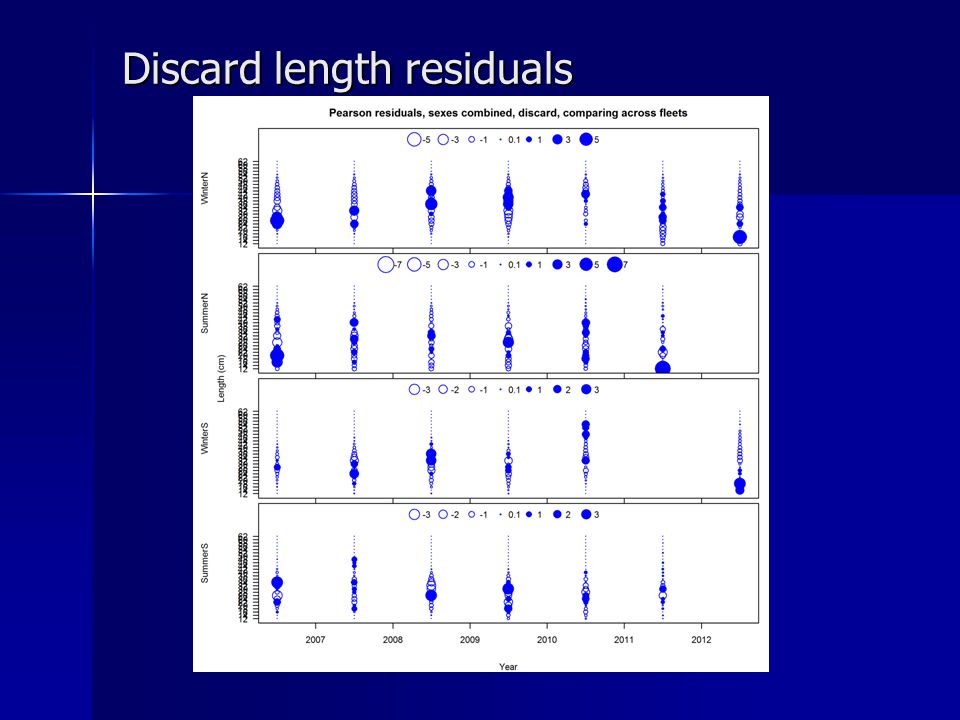
89. Discard length residuals

91. Tuning: Sigma R and Lengths Sigma R in = 0.40 Sigma R out = 0.35 LengthsAges Fleet Variance Adjustment MeaneffN MeaninputN Variance Adjustment MeaneffN MeaninputN Winter north 2.01.1 71.0 Summer north 1.41.0 1.71.0 Winter south 1.61.1 1.90.9 Summer south 1.21.0 1.41.1 Early Triennial 1.31.1 Late Triennial 1.01.1 NWFSC 1.00.9 0.30.7

92. Biomass trajectory Spawning Biomass Depletion Spawning Biomass Depletion

93. Recruitment deviations

94. Fishing mortality

95. Spawning potential ratio

96. Management performance

97. Retrospectives

98. Model Retrospectives Assessment YearBase20112010200920082007 SSB Unfished31,99831,80932,00732,43331,82832,196 2007 Depletion0.1430.1440.1460.1530.1510.160 2008 Depletion0.1340.1350.1380.1480.1470.162 2009 Depletion0.1290.1300.1350.1480.1500.172 2010 Depletion0.1260.1270.1320.1500.1620.183 2011 Depletion0.1560.1570.1640.1890.2090.219 2012 Depletion0.2060.2090.2200.2460.2610.254 2013 Depletion0.2750.2800.2870.3050.3020.280

99. Sensitivities Red-4 fleets w/ North comps Mirrored Green-6 fleets

100. Sensitivities: Removal of 2012 survey data Green-indexYellow-Ages Red-Lengths

101. Likelihood Profiles

103. Between Assessment Model Comparison 1999 – Red 1999 – Red 2005 – Green 2005 – Green 2009 – Blue 2009 – Blue 2011 – Light Blue 2011 – Light Blue 2013 - Black 2013 - Black

104. Decision Table State of nature LowBase caseHigh M = 0.14M = 0.16M = 0.18 Relative probability0.250.50.25 Management decision Year Catch (mt) SB(mt)Depl SB (mt) DeplSB(mt)Depl OFL 2015 3,94411,5460.33411,9210.37312,3610.414 2016 3,91411,5680.33511,8470.37012,1980.409 2017 3,72211,0630.32011,2410.35111,4920.385 2018 3,48510,4220.30210,5260.32910,7020.359 2019 3,2799,8620.2869,9340.31010,0700.337 2020 3,1339,4460.2749,5230.2989,6510.323 2021 3,0439,1610.2659,2640.2909,4070.315 2022 2,9908,9670.2609,1080.2859,2730.311 2023 2,9588,8280.2569,0070.2819,1970.308 2024 2,9358,7210.2538,9340.2799,1420.306 Status quo catches 20152,592 11,5460.33411,9210.37312,3610.414 20162,592 12,3360.35712,6110.39412,9460.434 20172,592 12,6610.36712,8140.40013,0210.436 20182,592 12,7500.36912,7910.40012,8840.432 20192,592 12,7440.36912,7000.39712,7090.426 20202,592 12,7050.36812,6050.39412,5590.421 20212,592 12,6590.36712,5270.39112,4510.417 20222,592 12,6160.36512,4690.39012,3790.415 20232,592 12,5790.36412,4280.38812,3320.413 20242,592 12,5470.36312,3970.38712,3000.412